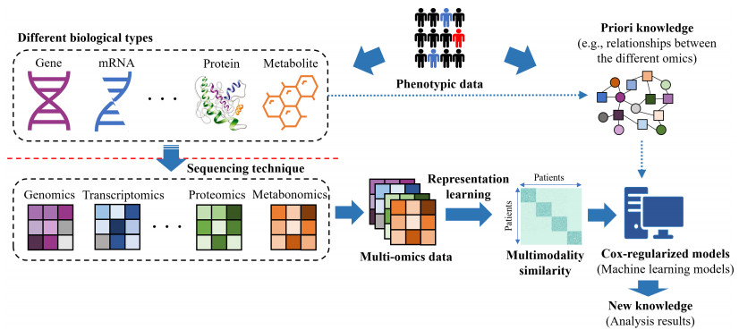
Cancer subtyping (or cancer subtypes identification) based on multi-omics data has played an important role in advancing diagnosis, prognosis and treatment, which triggers the development of advanced multi-view clustering algorithms. However, the high-dimension and heterogeneity of multi-omics data make great effects on the performance of these methods. In this paper, we propose to learn the informative latent representation based on autoencoder (AE) to naturally capture nonlinear omic features in lower dimensions, which is helpful for identifying the similarity of patients. Moreover, to take advantage of survival information or clinical information, a multi-omic survival analysis approach is embedded when integrating the similarity graph of heterogeneous data at the multi-omics level. Then, the clustering method is performed on the integrated similarity to generate subtype groups. In the experimental part, the effectiveness of the proposed framework is confirmed by evaluating five different multi-omics datasets, taken from The Cancer Genome Atlas. The results show that AE-assisted multi-omics clustering method can identify clinically significant cancer subtypes.
Citation: Shuwei Zhu, Wenping Wang, Wei Fang, Meiji Cui. Autoencoder-assisted latent representation learning for survival prediction and multi-view clustering on multi-omics cancer subtyping[J]. Mathematical Biosciences and Engineering, 2023, 20(12): 21098-21119. doi: 10.3934/mbe.2023933
Cancer subtyping (or cancer subtypes identification) based on multi-omics data has played an important role in advancing diagnosis, prognosis and treatment, which triggers the development of advanced multi-view clustering algorithms. However, the high-dimension and heterogeneity of multi-omics data make great effects on the performance of these methods. In this paper, we propose to learn the informative latent representation based on autoencoder (AE) to naturally capture nonlinear omic features in lower dimensions, which is helpful for identifying the similarity of patients. Moreover, to take advantage of survival information or clinical information, a multi-omic survival analysis approach is embedded when integrating the similarity graph of heterogeneous data at the multi-omics level. Then, the clustering method is performed on the integrated similarity to generate subtype groups. In the experimental part, the effectiveness of the proposed framework is confirmed by evaluating five different multi-omics datasets, taken from The Cancer Genome Atlas. The results show that AE-assisted multi-omics clustering method can identify clinically significant cancer subtypes.

| [1] |
A. Conesa, S. Beck, Making multi-omics data accessible to researchers, Sci. Data, 6 (2019), 251. https://doi.org/10.1038/s41597-019-0258-4 doi: 10.1038/s41597-019-0258-4

|
| [2] |
P. S. Reel, S. Reel, E. Pearson, E. Trucco, E. Jefferson, Using machine learning approaches for multi-omics data analysis: A review, Biotechnol. Adv., 49 (2021), 107739. https://doi.org/10.1016/j.biotechadv.2021.107739 doi: 10.1016/j.biotechadv.2021.107739
|
| [3] |
M. Zitnik, F. Nguyen, B. Wang, J. Leskovec, A. Goldenberg, M. M. Hoffman, Machine learning for integrating data in biology and medicine: Principles, practice, and opportunities, Inf. Fusion, 50 (2019), 71–91. https://doi.org/10.1016/j.inffus.2018.09.012 doi: 10.1016/j.inffus.2018.09.012
|
| [4] |
J. Lipkova, R. J. Chen, B. Chen, M. Y. Lu, M. Barbieri, D. Shao, et al., Artificial intelligence for multimodal data integration in oncology, Cancer Cell, 40 (2022), 1095–1110. https://doi.org/10.1016/j.ccell.2022.09.012 doi: 10.1016/j.ccell.2022.09.012
|
| [5] |
G. Cammarota, G. Ianiro, A. Ahern, C. Carbone, A. Temko, M. J. Claesson, et al., Gut microbiome, big data and machine learning to promote precision medicine for cancer, Nat. Rev. Gastroenterol. Hepatol., 17 (2020), 635–648. https://doi.org/10.1038/s41575-020-0327-3 doi: 10.1038/s41575-020-0327-3
|
| [6] |
N. Rappoport, R. Shamir, Multi-omic and multi-view clustering algorithms: review and cancer benchmark, Nucleic Acids Res., 46 (2018), 10546–10562. https://doi.org/10.1093/nar/gky889 doi: 10.1093/nar/gky889
|
| [7] | T. Ma, A. Zhang, Integrate multi-omic data using affinity network fusion (ANF) for cancer patient clustering, in 2017 IEEE International Conference on Bioinformatics and Biomedicine (BIBM), (2017), 398–403. https://doi.org/10.1109/BIBM.2017.8217682 |
| [8] |
Y. Guo, J. Zheng, X. Shang, Z. Li, A similarity regression fusion model for integrating multi-omics data to identify cancer subtypes, Genes, 9 (2018), 314. https://doi.org/10.3390/genes9070314 doi: 10.3390/genes9070314
|
| [9] |
H. Ding, M. Sharpnack, C. Wang, K. Huang, R. Machiraju, Integrative cancer patient stratification via subspace merging, Bioinformatics, 35 (2019), 1653–1659. https://doi.org/10.1093/bioinformatics/bty866 doi: 10.1093/bioinformatics/bty866
|
| [10] |
C. Chauvel, A. Novoloaca, P. Veyre, F. Reynier, J. Becker, Evaluation of integrative clustering methods for the analysis of multi-omics data, Briefings Bioinf., 21 (2020), 541–552. https://doi.org/10.1093/bib/bbz015 doi: 10.1093/bib/bbz015
|
| [11] |
B. Pfeifer, M. G. Schimek, A hierarchical clustering and data fusion approach for disease subtype discovery, J. Biomed. Inf., 113 (2021), 103636. https://doi.org/10.1016/j.jbi.2020.103636 doi: 10.1016/j.jbi.2020.103636
|
| [12] |
G. Brière, É. Darbo, P. Thébault, R. Uricaru, Consensus clustering applied to multi-omics disease subtyping, BMC Bioinf., 22 (2021), 1–29. https://doi.org/10.1186/s12859-021-04279-1 doi: 10.1186/s12859-021-04279-1
|
| [13] |
C. Liu, W. Cao, S. Wu, W. Shen, D. Jiang, Z. Yu, et al., Supervised graph clustering for cancer subtyping based on survival analysis and integration of multi-omic tumor data, IEEE/ACM Trans. Comput. Biol. Bioinf., 19 (2022), 1193–1202. https://doi.org/10.1109/TCBB.2020.3010509 doi: 10.1109/TCBB.2020.3010509
|
| [14] | Y. Li, J. Wang, J. Ye, C. K. Reddy, A multi-task learning formulation for survival analysis, in Proceedings of the 22nd ACM SIGKDD International Conference on Knowledge Discovery and Data Mining, (2016), 1715–1724. https://doi.org/10.1145/2939672.2939857 |
| [15] |
H. Chai, X. Zhou, Z. Zhang, J. Rao, H. Zhao, Y. Yang, Integrating multi-omics data through deep learning for accurate cancer prognosis prediction, Comput. Biol. Med., 134 (2021), 104481. https://doi.org/10.1016/j.compbiomed.2021.104481 doi: 10.1016/j.compbiomed.2021.104481
|
| [16] |
C. Liu, S. Wu, D. Jiang, Z. Yu, H. S. Wong, View-aware collaborative learning for survival prediction and subgroup identification, IEEE Trans. Biomed. Eng., 70 (2022), 307–317. https://doi.org/10.1109/TBME.2022.3190050 doi: 10.1109/TBME.2022.3190050
|
| [17] |
J. Zhao, X. Xie, X. Xu, S. Sun, Multi-view learning overview: Recent progress and new challenges, Inf. Fusion, 38 (2017), 43–54. https://doi.org/10.1016/j.inffus.2017.02.007 doi: 10.1016/j.inffus.2017.02.007
|
| [18] |
Z. Huang, J. Wu, A multiview clustering method with low-rank and sparsity constraints for cancer subtyping, IEEE/ACM Trans. Comput. Biol. Bioinf., 19 (2022), 3213–3223. https://doi.org/10.1109/TCBB.2021.3122917 doi: 10.1109/TCBB.2021.3122917
|
| [19] |
Z. Chen, Z. Yang, L. Zhu, P. Gao, T. Matsubara, S. Kanaya, M. Altaf-Ul-Amin, Learning vector quantized representation for cancer subtypes identification, Comput. Methods Programs Biomed., 236 (2023), 107543. https://doi.org/10.1016/j.cmpb.2023.107543 doi: 10.1016/j.cmpb.2023.107543
|
| [20] |
S. Ge, J. Liu, Y. Cheng, X. Meng, X. Wang, Multi-view spectral clustering with latent representation learning for applications on multi-omics cancer subtyping, Briefings Bioinf., 24 (2023), bbac500. https://doi.org/10.1093/bib/bbac500 doi: 10.1093/bib/bbac500
|
| [21] |
J. Zhao, B. Zhao, X. Song, C. Lyu, W. Chen, Y. Xiong, et al., Subtype-DCC: decoupled contrastive clustering method for cancer subtype identification based on multi-omics data, Brief. Bioinf., 24 (2023), bbad025. https://doi.org/10.1093/bib/bbad025 doi: 10.1093/bib/bbad025
|
| [22] |
X. Ye, Y. Shang, T. Shi, W. Zhang, T. Sakurai, Multi-omics clustering for cancer subtyping based on latent subspace learning, Comput. Biol. Med., 164 (2023), 107223. https://doi.org/10.1016/j.compbiomed.2023.107223 doi: 10.1016/j.compbiomed.2023.107223
|
| [23] |
C. Zhang, Y. Chen, T. Zeng, C. Zhang, L. Chen, Deep latent space fusion for adaptive representation of heterogeneous multi-omics data, Briefings Bioinf., 23 (2022), bbab600. https://doi.org/10.1093/bib/bbab600 doi: 10.1093/bib/bbab600
|
| [24] |
L. Zong, X. Zhang, L. Zhao, H. Yu, Q. Zhao, Multi-view clustering via multi-manifold regularized non-negative matrix factorization, Neural Networks, 88 (2017), 74–89. https://doi.org/10.1016/j.neunet.2017.02.003 doi: 10.1016/j.neunet.2017.02.003
|
| [25] |
X. Li, H. Zhang, R. Wang, F. Nie, Multiview clustering: A scalable and parameter-free bipartite graph fusion method, IEEE Trans. Pattern Anal. Mach. Intell., 44 (2022), 330–344. https://doi.org/10.1109/TPAMI.2020.3011148 doi: 10.1109/TPAMI.2020.3011148
|
| [26] |
Y. Pan, C. Q. Huang, D. Wang, Multiview spectral clustering via robust subspace segmentation, IEEE Trans. Cybern., 52 (2022), 2467–2476. https://doi.org/10.1109/TCYB.2020.3004220 doi: 10.1109/TCYB.2020.3004220
|
| [27] |
H. Wang, Y. Yang, B. Liu, GMC: Graph-based multi-view clustering, IEEE Trans. Knowl. Data Eng., 32 (2019), 1116–1129. https://doi.org/10.1109/TKDE.2019.2903810 doi: 10.1109/TKDE.2019.2903810
|
| [28] |
B. B. Avants, N. J. Tustison, J. R. Stone, Similarity-driven multi-view embeddings from highdimensional biomedical data, Nat. Comput. Sci., 1 (2021), 143–152. https://doi.org/10.1038/s43588-021-00029-8 doi: 10.1038/s43588-021-00029-8
|
| [29] |
Z. Zhao, M. Zhou, S. Liu, Iterated greedy algorithms for flow-shop scheduling problems: A tutorial, IEEE Trans. Autom. Sci. Eng., 19 (2021), 1941–1959. https://doi.org/10.1109/TASE.2021.3062994 doi: 10.1109/TASE.2021.3062994
|
| [30] |
S. Zhu, L. Xu, E. D. Goodman, Z. Lu, A new many-objective evolutionary algorithm based on generalized pareto dominance, IEEE Trans. Cybern., 52 (2022), 7776–7790. https://doi.org/10.1109/TCYB.2021.3051078 doi: 10.1109/TCYB.2021.3051078
|
| [31] |
M. Cui, L. Li, M. Zhou, A. Abusorrah, Surrogate-assisted autoencoder-embedded evolutionary optimization algorithm to solve high-dimensional expensive problems, IEEE Trans. Evol. Comput., 26 (2022), 676–689. https://doi.org/10.1109/TEVC.2021.3113923 doi: 10.1109/TEVC.2021.3113923
|
| [32] |
M. Cui, L. Li, M. Zhou, J. Li, A. Abusorrah, K. Sedraoui, A bi-population cooperative optimization algorithm assisted by an autoencoder for medium-scale expensive problems, IEEE/CAA J. Autom. Sin., 9 (2022), 1952–1966. https://doi.org/10.1109/JAS.2022.105425 doi: 10.1109/JAS.2022.105425
|
| [33] |
R. Tibshirani, The lasso method for variable selection in the Cox model, Stat. Med., 16 (1997), 385–395. https://doi.org/10.1002/(SICI)1097-0258(19970228)16:4%3C385::AID-SIM380%3E3.0.CO;2-3 doi: 10.1002/(SICI)1097-0258(19970228)16:4%3C385::AID-SIM380%3E3.0.CO;2-3
|
| [34] | J. Zhang, J. Huan, Inductive multi-task learning with multiple view data, in Proceedings of the 18th ACM SIGKDD International Conference on Knowledge Discovery and Data Mining, (2012), 543–551. https://doi.org/10.1145/2339530.2339617 |
| [35] | F. Nie, X. Wang, M. Jordan, H. Huang, The constrained laplacian rank algorithm for graph-based clustering, in Proceedings of the AAAI Conference on Artificial Intelligence, 30 (2016), 1969–1976. https://doi.org/10.1609/aaai.v30i1.10302 |
| [36] |
A. Beck, M. Teboulle, A fast iterative shrinkage-thresholding algorithm for linear inverse problems, SIAM J. Imaging Sci., 2 (2009), 183–202. https://doi.org/10.1137/08071654 doi: 10.1137/08071654
|
| [37] | X. Guo, Robust subspace segmentation by simultaneously learning data representations and their affinity matrix, in Twenty-fourth International Joint Conference on Artificial Intelligence, (2015), 3547–3553. https://dl.acm.org/doi/abs/10.5555/2832581.2832743 |
| [38] |
S. Zhu, L. Xu, E. D. Goodman, Hierarchical topology-based cluster representation for scalable evolutionary multiobjective clustering, IEEE Trans. Cybern., 52 (2022), 9846–9860. https://doi.org/10.1109/TCYB.2021.3081988 doi: 10.1109/TCYB.2021.3081988
|
| [39] |
S. Zhu, L. Xu, E. D. Goodman, Evolutionary multi-objective automatic clustering enhanced with quality metrics and ensemble strategy, Knowledge-Based Syst., 188 (2020), 105018. https://doi.org/10.1016/j.knosys.2019.105018 doi: 10.1016/j.knosys.2019.105018
|
| [40] |
A. L. Fred, A. K. Jain, Combining multiple clusterings using evidence accumulation, IEEE Trans. Pattern Anal. Mach. Intell., 27 (2005), 835–850. https://doi.org/10.1109/TPAMI.2005.113 doi: 10.1109/TPAMI.2005.113
|
| [41] |
A. Strehl, J. Ghosh, Cluster ensembles–-a knowledge reuse framework for combining multiple partitions, J. Mach. Learn. Res., 3 (2002), 583–617. https://doi.org/10.1162/153244303321897735 doi: 10.1162/153244303321897735
|
| [42] |
D. Huang, C. D. Wang, J. H. Lai, Locally weighted ensemble clustering, IEEE Trans. Cybern., 5 (2018), 1460–1473. https://doi.org/10.1109/TCYB.2017.2702343 doi: 10.1109/TCYB.2017.2702343
|
| [43] |
S. Paul, Capturing the latent space of an autoencoder for multi-omics integration and cancer subtyping, Comput. Biol. Med., 148 (2022), 105832. https://doi.org/10.1016/j.compbiomed.2022.105832 doi: 10.1016/j.compbiomed.2022.105832
|
| [44] |
Y. Perez-Riverol, M. Bai, F. da Veiga Leprevost, S. Squizzato, Y. M. Park, K. Haug, et al., Discovering and linking public omics data sets using the omics discovery index, Nat. Biotechnol., 35 (2017), 406–409. https://doi.org/10.1038/nbt.3790 doi: 10.1038/nbt.3790
|
| [45] |
P. L. Triozzi, E. R. Stirling, Q. Song, B. Westwood, M. Kooshki, M. E. Forbes, et al., Circulating immune bioenergetic, metabolic, and genetic signatures predict melanoma patients' response to anti–pd-1 immune checkpoint blockade, Clin. Cancer Res., 28 (2022), 1192–1202. https://doi.org/10.1158/1078-0432.CCR-21-3114 doi: 10.1158/1078-0432.CCR-21-3114
|
| [46] |
A. K. Pullikuth, E. D. Routh, K. D. Zimmerman, J. Chifman, J. W. Chou, M. H. Soike, et al., Bulk and single-cell profiling of breast tumors identifies trem-1 as a dominant immune suppressive marker associated with poor outcomes, Front. Oncol., 11 (2021), 734959. https://doi.org/10.3389/fonc.2021.734959 doi: 10.3389/fonc.2021.734959
|
| [47] |
B. Wang, A. M. Mezlini, F. Demir, M. Fiume, Z. Tu, M. Brudno, et al., Similarity network fusion for aggregating data types on a genomic scale, Nat. Methods, 11 (2014), 333–337. https://doi.org/10.1038/nmeth.2810 doi: 10.1038/nmeth.2810
|
| [48] |
H. Torkey, M. Atlam, N. El-Fishawy, H. Salem, A novel deep autoencoder based survival analysis approach for microarray dataset, PeerJ Comput. Sci., 7 (2021), e492. https://doi.org/10.7717/peerj-cs.492 doi: 10.7717/peerj-cs.492
|
| [49] |
P. J. Rousseeuw, Silhouettes: a graphical aid to the interpretation and validation of cluster analysis, J. Comput. Appl. Math., 20 (1987), 53–65. https://doi.org/10.1016/0377-0427(87)90125-7 doi: 10.1016/0377-0427(87)90125-7
|
| [50] |
S. Zhu, L. Xu, Many-objective fuzzy centroids clustering algorithm for categorical data, Expert Syst. Appl., 96 (2018), 230–248. https://doi.org/10.1016/j.eswa.2017.12.013 doi: 10.1016/j.eswa.2017.12.013
|
| [51] |
Z. Lu, I. Whalen, Y. Dhebar, K. Deb, E. Goodman, W. Banzhaf, et al., Multi-objective evolutionary design of deep convolutional neural networks for image classification, IEEE Trans. Evol. Comput., 25 (2020), 277–291. https://doi.org/10.1109/TEVC.2020.3024708 doi: 10.1109/TEVC.2020.3024708
|
| [52] | Z. Lu, G. Sreekumar, E. Goodman, W. Banzhaf, K. Deb, V. N. Boddeti, Neural architecture transfer, IEEE Trans. Pattern Anal. Mach. Intell., 43 (2021), 2971–2989. https://doi.org/10.1109/TPAMI.2021.3052758 |


Figures(8) / Tables(4)

Shuwei Zhu, Wenping Wang, Wei Fang, Meiji Cui. Autoencoder-assisted latent representation learning for survival prediction and multi-view clustering on multi-omics cancer subtyping[J]. Mathematical Biosciences and Engineering, 2023, 20(12): 21098-21119. doi: 10.3934/mbe.2023933


 DownLoad: