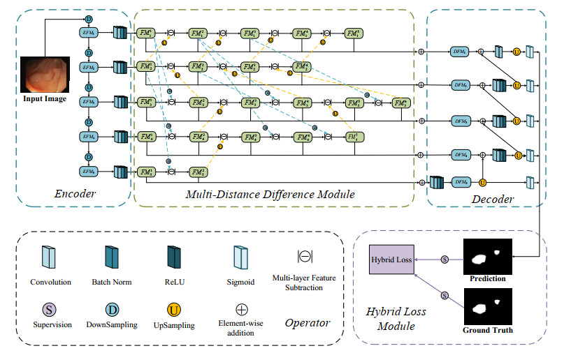
Colorectal malignancies often arise from adenomatous polyps, which typically begin as solitary, asymptomatic growths before progressing to malignancy. Colonoscopy is widely recognized as a highly efficacious clinical polyp detection method, offering valuable visual data that facilitates precise identification and subsequent removal of these tumors. Nevertheless, accurately segmenting individual polyps poses a considerable difficulty because polyps exhibit intricate and changeable characteristics, including shape, size, color, quantity and growth context during different stages. The presence of similar contextual structures around polyps significantly hampers the performance of commonly used convolutional neural network (CNN)-based automatic detection models to accurately capture valid polyp features, and these large receptive field CNN models often overlook the details of small polyps, which leads to the occurrence of false detections and missed detections. To tackle these challenges, we introduce a novel approach for automatic polyp segmentation, known as the multi-distance feature dissimilarity-guided fully convolutional network. This approach comprises three essential components, i.e., an encoder-decoder, a multi-distance difference (MDD) module and a hybrid loss (HL) module. Specifically, the MDD module primarily employs a multi-layer feature subtraction (MLFS) strategy to propagate features from the encoder to the decoder, which focuses on extracting information differences between neighboring layers' features at short distances, and both short and long-distance feature differences across layers. Drawing inspiration from pyramids, the MDD module effectively acquires discriminative features from neighboring layers or across layers in a continuous manner, which helps to strengthen feature complementary across different layers. The HL module is responsible for supervising the feature maps extracted at each layer of the network to improve prediction accuracy. Our experimental results on four challenge datasets demonstrate that the proposed approach exhibits superior automatic polyp performance in terms of the six evaluation criteria compared to five current state-of-the-art approaches.
Citation: Nan Mu, Jinjia Guo, Rong Wang. Automated polyp segmentation based on a multi-distance feature dissimilarity-guided fully convolutional network[J]. Mathematical Biosciences and Engineering, 2023, 20(11): 20116-20134. doi: 10.3934/mbe.2023891
Colorectal malignancies often arise from adenomatous polyps, which typically begin as solitary, asymptomatic growths before progressing to malignancy. Colonoscopy is widely recognized as a highly efficacious clinical polyp detection method, offering valuable visual data that facilitates precise identification and subsequent removal of these tumors. Nevertheless, accurately segmenting individual polyps poses a considerable difficulty because polyps exhibit intricate and changeable characteristics, including shape, size, color, quantity and growth context during different stages. The presence of similar contextual structures around polyps significantly hampers the performance of commonly used convolutional neural network (CNN)-based automatic detection models to accurately capture valid polyp features, and these large receptive field CNN models often overlook the details of small polyps, which leads to the occurrence of false detections and missed detections. To tackle these challenges, we introduce a novel approach for automatic polyp segmentation, known as the multi-distance feature dissimilarity-guided fully convolutional network. This approach comprises three essential components, i.e., an encoder-decoder, a multi-distance difference (MDD) module and a hybrid loss (HL) module. Specifically, the MDD module primarily employs a multi-layer feature subtraction (MLFS) strategy to propagate features from the encoder to the decoder, which focuses on extracting information differences between neighboring layers' features at short distances, and both short and long-distance feature differences across layers. Drawing inspiration from pyramids, the MDD module effectively acquires discriminative features from neighboring layers or across layers in a continuous manner, which helps to strengthen feature complementary across different layers. The HL module is responsible for supervising the feature maps extracted at each layer of the network to improve prediction accuracy. Our experimental results on four challenge datasets demonstrate that the proposed approach exhibits superior automatic polyp performance in terms of the six evaluation criteria compared to five current state-of-the-art approaches.

| [1] |
E. Morgan, M. Arnold, A. Gini1, V. Lorenzoni, C. J. Cabasag, M. Laversanne, et al., Global burden of colorectal cancer in 2020 and 2040: incidence and mortality estimates from GLOBOCAN, Gut, 72 (2023), 338–344. https://doi.org/10.1136/gutjnl-2022-327736 doi: 10.1136/gutjnl-2022-327736

|
| [2] |
L. Rabeneck, H. El-Serag, J. Davila, R. Sandler, Outcomes of colorectal cancer in the United States: no change in survival (1986–1997), Am. J. Gastroenterol., 98 (2003), 471–477. https://doi.org/10.1111/j.1572-0241.2003.07260.x doi: 10.1111/j.1572-0241.2003.07260.x
|
| [3] | J. Tang, S. Millington, S. T. Acton, J. Crandall, S. Hurwitz, Ankle cartilage surface segmentation using directional gradient vector flow snakes, in International Conference on Image Processing, (2004), 2745–2748. https://doi.org/10.1109/ICIP.2004.1421672 |
| [4] |
J. Tang, S. Guo, Q. Sun, Y. Deng, D. Zhou, Speckle reducing bilateral filter for cattle follicle segmentation, BMC Genomics, 11 (2010), 1–9. https://doi.org/10.1186/1471-2164-11-1 doi: 10.1186/1471-2164-11-1
|
| [5] | P. Brandao, E. Mazomenos, G. Ciuti, R. Caliò, F. Bianchi, A. Menciassi, et al., Fully convolutional neural networks for polyp segmentation in colonoscopy, in Medical Imaging 2017: Computer-Aided Diagnosis, 10134 (2017), 101–107. https://doi.org/10.1117/12.2254361 |
| [6] |
N. Mu, H. Wang, Y. Zhang, J. Jiang, J. Tang, Progressive global perception and local polishing network for lung infection segmentation of COVID-19 CT images, Pattern Recognit., 121 (2021), 1–12. https://doi.org/10.1016/j.patcog.2021.108168 doi: 10.1016/j.patcog.2021.108168
|
| [7] | O. Ronneberger, P. Fischer, T. Brox, U-net: Convolutional networks for biomedical image segmentation, in Medical Image Computing and Computer-Assisted Intervention, (2015), 234–241. https://doi.org/10.1007/978-3-319-24574-4_28 |
| [8] |
N. Mu, Z. Lyu, M. Rezaeitaleshmahalleh, J. Tang, J. Jiang, An attention residual u-net with differential preprocessing and geometric postprocessing: Learning how to segment vasculature including intracranial aneurysms, Med. Image Anal., 84 (2023), 1–12. https://doi.org/10.1016/j.media.2022.102697 doi: 10.1016/j.media.2022.102697
|
| [9] |
J. He, Q. Zhu, K. Zhang, P. Yu, J. Tang, An evolvable adversarial network with gradient penalty for COVID-19 infection segmentation, Appl. Soft Comput., 113 (2021), 1–10. https://doi.org/10.1016/j.asoc.2021.107947 doi: 10.1016/j.asoc.2021.107947
|
| [10] |
N. Mu, Z. Lyu, M. Rezaeitaleshmahalleh, X. Zhang, T. Rasmussen, R. McBane, et al., Automatic segmentation of abdominal aortic aneurysms from CT angiography using a context-aware cascaded U-Net, Comput. Biol. Med., 158 (2023), 1–11. https://doi.org/10.1016/j.compbiomed.2023.106569 doi: 10.1016/j.compbiomed.2023.106569
|
| [11] | N. Tajbakhsh, S. Gurudu, J. Liang, Automatic polyp detection in colonoscopy videos using an ensemble of convolutional neural networks, in IEEE 12th International Symposium on Biomedical Imaging, (2015), 79–83. https://doi.org/10.1109/ISBI.2015.7163821 |
| [12] |
Y. Shin, H. A. Qadir, L. Aabakken, J. Bergsland, I. Balasingham, Automatic colon polyp detection using region based deep CNN and post learning approaches, IEEE Access, 6 (2018), 40950–40962. https://doi.org/10.1109/ACCESS.2018.2856402 doi: 10.1109/ACCESS.2018.2856402
|
| [13] |
J. S. Nisha, V. P. Gopi, P. Palanisamy, Automated colorectal polyp detection based on image enhancement and dual-path CNN architecture, Biomed. Signal Process. Control, 73 (2022), 103465. https://doi.org/10.1016/j.bspc.2021.103465 doi: 10.1016/j.bspc.2021.103465
|
| [14] | G. Ji, Y. Chou, D. Fan, G. Chen, H. Fu, Progressively normalized self-attention network for video polyp segmentation, in International Conference on Medical Image Computing and Computer-Assisted Intervention, (2021), 142–152. https://doi.org/10.1007/978-3-030-87193-2_14 |
| [15] |
Y. Wen, L. Zhang, X. Meng, X. Ye, Rethinking the transfer learning for FCN based polyp segmentation in colonoscopy, IEEE Access, 11 (2023), 16183–16193. https://doi.org/10.1109/ACCESS.2023.3245519 doi: 10.1109/ACCESS.2023.3245519
|
| [16] | E. Sanderson, B. J. Matuszewski, FCN-transformer feature fusion for polyp segmentation, in Annual Conference on Medical Image Understanding and Analysis, (2022), 892–907. https://doi.org/10.1007/978-3-031-12053-4_65 |
| [17] | Z. Zhou, M. Siddiquee, N. Tajbakhsh, J. Liang, UNet++: A nested U-Net architecture for medical image segmentation, in Deep Learning in Medical Image Analysis and Multimodal Learning for Clinical Decision Support: 4th International Workshop, (2018), 3–11. https://doi.org/10.1007/978-3-030-00889-5_1 |
| [18] | D. Jha, P. Smedsrud, M. Riegler, D. Johansen, T. De Lange, Resunet++: An advanced architecture for medical image segmentation, in IEEE International Symposium on Multimedia, (2019), 225–230. https://doi.org/10.1109/ISM46123.2019.00049 |
| [19] | D. P. Fan, G. Ji, T. Zhou, G. Chen, H. Fu, Pranet: Parallel reverse attention network for polyp segmentation, in Medical Image Computing and Computer Assisted Intervention, (2020), 263–273. https://doi.org/10.1007/978-3-030-59725-2_26 |
| [20] | X. Zhao, L. Zang, H. Lu, Automatic polyp segmentation via multi-scale subtraction network, in Medical Image Computing and Computer Assisted Intervention, (2021), 120–130. https://doi.org/10.1007/978-3-030-87193-2_12 |
| [21] |
H. Wu, Z. Zhao, Z. Wang, META-Unet: Multi-scale efficient transformer attention Unet for fast and high-accuracy polyp segmentation, IEEE Trans. Autom. Sci. Eng., 2023 (2023), 1–12. https://doi.org/10.1109/TASE.2023.3292373 doi: 10.1109/TASE.2023.3292373
|
| [22] |
J. Lewis, Y. J. Cha, J. Kim, Dual encoder–decoder-based deep polyp segmentation network for colonoscopy images, Sci. Rep., 13 (2023), 1–12. https://doi.org/10.1038/s41598-022-26890-9 doi: 10.1038/s41598-022-26890-9
|
| [23] |
S. Gao, M. Cheng, K. Zhao, X. Zhang, M. Yang, Res2net: A new multi-scale backbone architecture, IEEE Trans. Pattern Anal. Mach. Intell., 43 (2019), 652–662. https://doi.org/10.1109/TPAMI.2019.2938758 doi: 10.1109/TPAMI.2019.2938758
|
| [24] |
N. Tajbakhsh, S. R. Gurudu, J. Liang, Automated polyp detection in colonoscopy videos using shape and context information, IEEE Trans. Med. Imaging, 35 (2015), 630–644. https://doi.org/10.1109/TMI.2015.2487997 doi: 10.1109/TMI.2015.2487997
|
| [25] |
J. Bernal, F. Sánchez, G. Fernández-Esparrach, D. Gil, C. Rodríguez, WM-DOVA maps for accurate polyp highlighting in colonoscopy: Validation vs. saliency maps from physicians, Comput. Med. Imaging Graphics, 43 (2015), 99–111. https://doi.org/10.1016/j.compmedimag.2015.02.007 doi: 10.1016/j.compmedimag.2015.02.007
|
| [26] |
D. Vázquez, J. Bernal, F. J. Sánchez, G. Fernández-Esparrach, A. M. López, A. Romero, et al., A benchmark for endoluminal scene segmentation of colonoscopy images, J. Healthcare Eng., 2017 (2017), 1–10. https://doi.org/10.1155/2017/4037190 doi: 10.1155/2017/4037190
|
| [27] | D. Jha, P. H. Smedsrud, M. A. Riegler, P. Halvorsen, T. D. Lange, D. Johansen, et al., Kvasir-seg: A segmented polyp dataset, in MMM: 26th International Conference, (2020), 451–462. https://doi.org/10.1007/978-3-030-37734-2_37 |
| [28] | R. Margolin, L. Zelnik-Manor, A. Tal, How to evaluate foreground maps? in IEEE Conference on Computer Vision and Pattern Recognition, (2014), 248–255. https://doi.org/10.1109/CVPR.2014.39 |
| [29] | D. P. Fan, M. Cheng, Y. Liu, T. Li, A. Borji, Structure-measure: A new way to evaluate foreground maps, in Proceedings of the IEEE International Conference on Computer Vision, (2017), 4548–4557. |
| [30] | D. P. Fan, C. Gong, Y. Cao, B. Ren, M. M. Cheng, A. Borji, Enhanced-alignment measure for binary foreground map evaluation, in International Joint Conference on Artificial Intelligence, (2018), 1–7. |
| [31] |
D. P. Fan, T. Zhou, G. Ji, Y. Zhou, G. Chen, Inf-net: Automatic COVID-19 lung infection segmentation from CT images, IEEE Trans. Med. Imaging, 39 (2020), 2626–2637. https://doi.org/10.1109/TMI.2020.2996645 doi: 10.1109/TMI.2020.2996645
|
| [32] | S. Yu, J. Xiao, B. Zhang, E. Lim, Democracy does matter: Comprehensive feature mining for co-salient object detection, in IEEE/CVF Conference on Computer Vision and Pattern Recognition, (2022), 979–988. |
| [33] | Y. Wang, W. Zang, L. Wang, T. Liu, H. Lu, Multi-source uncertainty mining for deep unsupervised saliency detection, in IEEE/CVF Conference on Computer Vision and Pattern Recognition, (2022), 11727–11736. https://doi.org/10.1109/CVPR52688.2022.01143 |


Figures(4) / Tables(8)

Nan Mu, Jinjia Guo, Rong Wang. Automated polyp segmentation based on a multi-distance feature dissimilarity-guided fully convolutional network[J]. Mathematical Biosciences and Engineering, 2023, 20(11): 20116-20134. doi: 10.3934/mbe.2023891


 DownLoad: