Aspect-based sentiment analysis (ABSA) is a fine-grained and diverse task in natural language processing. Existing deep learning models for ABSA face the challenge of balancing the demand for finer granularity in sentiment analysis with the scarcity of training corpora for such granularity. To address this issue, we propose an enhanced BERT-based model for multi-dimensional aspect target semantic learning. Our model leverages BERT's pre-training and fine-tuning mechanisms, enabling it to capture rich semantic feature parameters. In addition, we propose a complex semantic enhancement mechanism for aspect targets to enrich and optimize fine-grained training corpora. Third, we combine the aspect recognition enhancement mechanism with a CRF model to achieve more robust and accurate entity recognition for aspect targets. Furthermore, we propose an adaptive local attention mechanism learning model to focus on sentiment elements around rich aspect target semantics. Finally, to address the varying contributions of each task in the joint training mechanism, we carefully optimize this training approach, allowing for a mutually beneficial training of multiple tasks. Experimental results on four Chinese and five English datasets demonstrate that our proposed mechanisms and methods effectively improve ABSA models, surpassing some of the latest models in multi-task and single-task scenarios.
Citation: Quan Zhu, Xiaoyin Wang, Xuan Liu, Wanru Du, Xingxing Ding. Multi-task learning for aspect level semantic classification combining complex aspect target semantic enhancement and adaptive local focus[J]. Mathematical Biosciences and Engineering, 2023, 20(10): 18566-18591. doi: 10.3934/mbe.2023824
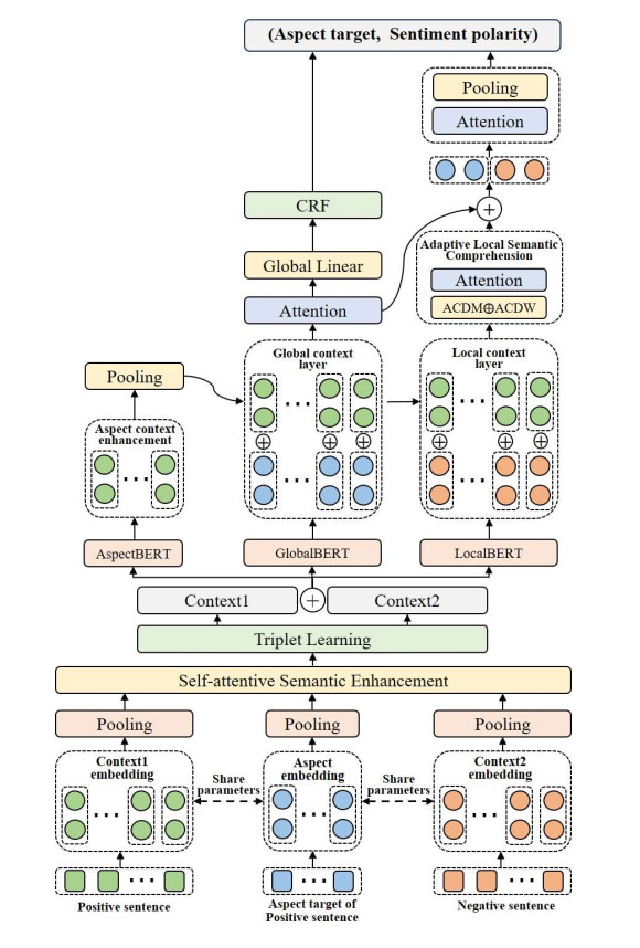
Aspect-based sentiment analysis (ABSA) is a fine-grained and diverse task in natural language processing. Existing deep learning models for ABSA face the challenge of balancing the demand for finer granularity in sentiment analysis with the scarcity of training corpora for such granularity. To address this issue, we propose an enhanced BERT-based model for multi-dimensional aspect target semantic learning. Our model leverages BERT's pre-training and fine-tuning mechanisms, enabling it to capture rich semantic feature parameters. In addition, we propose a complex semantic enhancement mechanism for aspect targets to enrich and optimize fine-grained training corpora. Third, we combine the aspect recognition enhancement mechanism with a CRF model to achieve more robust and accurate entity recognition for aspect targets. Furthermore, we propose an adaptive local attention mechanism learning model to focus on sentiment elements around rich aspect target semantics. Finally, to address the varying contributions of each task in the joint training mechanism, we carefully optimize this training approach, allowing for a mutually beneficial training of multiple tasks. Experimental results on four Chinese and five English datasets demonstrate that our proposed mechanisms and methods effectively improve ABSA models, surpassing some of the latest models in multi-task and single-task scenarios.

| [1] |
B. Pang, L. Lee, Opinion mining and sentiment analysis, Trends Inf. Retr., 2 (2008), 1–135. https://doi.org/10.1561/1500000011 doi: 10.1561/1500000011

|
| [2] |
G. Vinodhini, R. Chandrasekaran, Sentiment analysis and opinion mining: a survey, Int. J., 2 (2012), 282–292. https://doi.org/10.1016/j.nlp.2022.100003 doi: 10.1016/j.nlp.2022.100003
|
| [3] | M. Pontiki, D. Galanis, J. Pavlopoulos, H. Papageorgiou, S. Manandhar, SemEval-2014 Task 4: Aspect based sentiment analysis, in Association for Computational Linguistics, (2014), 27–35. https://doi.org/10.3115/v1/S14-2004 |
| [4] | M. Pontiki, D. Galanis, H. Papageorgiou, S. Manandhar, I. Androutsopoulos, Semeval-2015 task 12: Aspect based sentiment analysis, in Association for Computational Linguistics, (2015), 486–495. https://doi.org/10.18653/v1/S15-2082 |
| [5] | M. Pontiki, D. Galanis, H. Papageorgiou, I. Androutsopoulos, S. Manandhar, M. AL-Smadi, et al. Semeval-2016 task 5: Aspect based sentiment analysis, in Association for Computational Linguistics, (2016), 19–30. https://doi.org/10.18653/v1/S16-1002 |
| [6] |
W. Zhang, X. Li, Y. Deng, L. Bing, W. Lam, A survey on aspect-based sentiment analysis: Tasks, methods, and challenges, IEEE Trans. Knowl. Data Eng., 2022. https://doi.org/10.1109/TKDE.2022.3230975 doi: 10.1109/TKDE.2022.3230975
|
| [7] | D. Tang, B. Qin, X. Feng, T. Liu, Effective LSTMs for target-dependent sentiment classification, preprint, arXiv: 151201100. |
| [8] | M. Yang, W. Tu, J. Wang, F. Xu, X. Chen, Attention based LSTM for target dependent sentiment classification, in Proceedings of the AAAI conference on artificial intelligence, 2017. https://doi.org/10.1609/aaai.v31i1.11061 |
| [9] | Q. Liu, Y. Huang, Q. Yang, H. Peng, J. Wang, An attention-aware long short-term memory-like spiking neural model for sentiment analysis, Int. J. Neural Syst., (2023), 2350037–2350037. https://doi.org/10.1142/s0129065723500375 |
| [10] |
Y. Huang, Q. Liu, H. Peng, J. Wang, Q. Yang, D. Orellana-Martín, Sentiment classification using bidirectional LSTM-SNP model and attention mechanism, Expert Syst. Appl., 221 (2023), 119730. https://doi.org/10.1016/j.eswa.2023.119730 doi: 10.1016/j.eswa.2023.119730
|
| [11] |
Y. Huang, H. Peng, Q. Liu, Q. Yang, J. Wang, D. Orellana-Martín, et al., Attention-enabled gated spiking neural P model for aspect-level sentiment classification, Neural Network, 157 (2023), 437–443. https://doi.org/10.1016/j.neunet.2022.11.006 doi: 10.1016/j.neunet.2022.11.006
|
| [12] | Y. Kim, Convolutional neural networks for sentence classification, preprint, arXiv: 14085882. |
| [13] | D. Tang, B. Qin, T. Liu, Aspect level sentiment classification with deep memory network, preprint, arXiv: 160508900. |
| [14] | P. Lin, M. Yang, J. Lai. Deep mask memory network with semantic dependency and context moment for aspect level sentiment classification, in IJCAI, (2019), 5088–5094. https://doi.org/10.24963/ijcai.2019/707 |
| [15] | A. Vaswani, N. Shazeer, N. Parmar, J. Uszkoreit, L. Jones, A. N. Gomez, et al., Attention is all you need, in Advances in Neural Information Processing Systems, 30 (2017). https://doi.org/10.48550/arXiv.1706.03762 |
| [16] | Z.-Y. Dou, Capturing user and product information for document level sentiment analysis with deep memory network, in Proceedings of the 2017 Conference on Empirical Methods in Natural Language Processing, 2017. https://doi.org/10.18653/v1/D17-1054 |
| [17] |
K. Chakraborty, S. Bhattacharyya, R. Bag, A survey of sentiment analysis from social media data, IEEE Trans. Comput. Soc. Syst., 7 (2020), 450–464. https://doi.org/10.1109/TCSS.2019.2956957 doi: 10.1109/TCSS.2019.2956957
|
| [18] |
X. Zhu, Y. Zhu, L. Zhang, Y. Chen, A BERT-based multi-semantic learning model with aspect-aware enhancement for aspect polarity classification, Appl. Intell., 53 (2023), 4609–4623. https://doi.org/10.1007/s10489-022-03702-1 doi: 10.1007/s10489-022-03702-1
|
| [19] | J. Devlin, M. W. Chang, K. Lee, K. Toutanova, Bert: Pre-training of deep bidirectional transformers for language understanding, preprint, arXiv: 181004805. |
| [20] | N. Reimers, I. Gurevych, Sentence-bert: Sentence embeddings using siamese bert-networks, preprint, arXiv: 190810084. |
| [21] |
L. Breiman, J. Friedman, C. J. Stone, R. A. Olshen, Classification and Regression Trees (CART), Biometrics, 1984 (1984). https://doi.org/10.2307/2530946 doi: 10.2307/2530946
|
| [22] |
N. S. Altman, An introduction to kernel and nearest-neighbor nonparametric regression, Am. Stat., 46 (1992), 175–185. https://doi.org/10.1080/00031305.1992.10475879 doi: 10.1080/00031305.1992.10475879
|
| [23] | I. Rish, An empirical study of the naive Bayes classifier, in IJCAI 2001 workshop on empirical methods in artificial intelligence, (2001), 41–46. https://doi.org/10.1109/CSCI46756.2018.00065 |
| [24] | D. W. Hosmer Jr, S. Lemeshow, R. X. Sturdivant, Applied Logistic Regression, John Wiley & Sons, 2013. https://doi.org/10.1002/9781118548387 |
| [25] | C. Cortes, V. Vapnik, Support-vector networks, Mach. Learn., 20 (1995), 273–297. |
| [26] |
L. Breiman, Random forests, Mach. Learn., 45 (2001), 5–32. https://doi.org/10.1023/A:1022627411411 doi: 10.1023/A:1022627411411
|
| [27] | N. S. Joshi, S. A. Itkat, A survey on feature level sentiment analysis, Int. J. Comput. Sci. Inf. Technol., 5 (2014), 5422–5425. |
| [28] |
E. Cambria, B. White, Jumping NLP curves: A review of natural language processing research, IEEE Comput. Intell. Mag., 9 (2014), 48–57. https://doi.org/10.1109/MCI.2014.2307227 doi: 10.1109/MCI.2014.2307227
|
| [29] |
B. Zhang, X. Fu, C. Luo, Y. Ye, X. Li, L. Jing, Cross-domain aspect-based sentiment classification by exploiting domain-invariant semantic-primary feature, IEEE Trans. Affect. Comput., 2023 (2023), forthcoming. https://doi.org/10.1109/TAFFC.2023.3239540 doi: 10.1109/TAFFC.2023.3239540
|
| [30] |
H. Huang, B. Zhang, L. Jing, X. Fu, X. Chen, J. Shi, Logic tensor network with massive learned knowledge for aspect-based sentiment analysis, Knowl. Based Syst., 257 (2022), 109943. https://doi.org/10.1016/j.knosys.2022.109943 doi: 10.1016/j.knosys.2022.109943
|
| [31] |
X. Mei, Y. Zhou, C. Zhu, M. Wu, M. Li, S. Pan, A disentangled linguistic graph model for explainable aspect-based sentiment analysis, Knowl. Based Syst, 260 (2023), 110150. https://doi.org/10.1016/j.knosys.2022.110150 doi: 10.1016/j.knosys.2022.110150
|
| [32] | B. Zhang, X. Huang, Z. Huang, H. Huang, B. Zhang, X. Fu, et al., Sentiment interpretable logic tensor network for aspect-term sentiment analysis, in Proceedings of the 29th International Conference on Computational Linguistics, (2022), 6705–6714. |
| [33] | B. Xu, X. Wang, B. Yang, Z. Kang, Target embedding and position attention with lstm for aspect based sentiment analysis, in Proceedings of the 2020 5th International Conference on Mathematics and Artificial Intelligence, (2020), 93–97. https://doi.org/10.1145/3395260.3395280 |
| [34] | Y. Ma, H. Peng, E. Cambria, Targeted aspect-based sentiment analysis via embedding commonsense knowledge into an attentive LSTM, in Proceedings of the AAAI conference on artificial intelligence, (2018). https://doi.org/10.1609/aaai.v32i1.12048 |
| [35] | L. Bao, P. Lambert, T. Badia, Attention and lexicon regularized LSTM for aspect-based sentiment analysis, in Proceedings of the 57th annual meeting of the association for computational linguistics: student research workshop, (2019), 253–259. https://doi.org/10.18653/v1/P19-2035 |
| [36] |
Y. Xing, C. Xiao, Y. Wu, Z. Ding, A convolutional neural network for aspect-level sentiment classification, Int. J. Pattern Recognit. Artif Intell., 33 (2019), 1959046. https://doi.org/10.18653/v1/2021.textgraphs-1.8 doi: 10.18653/v1/2021.textgraphs-1.8
|
| [37] |
X. Wang, F. Li, Z. Zhang, G. Xu, J. Zhang, X. Sun, A unified position-aware convolutional neural network for aspect based sentiment analysis, Neurocomputing, 450 (2021), 91–103. https://doi.org/10.1016/j.neucom.2021.03.092 doi: 10.1016/j.neucom.2021.03.092
|
| [38] |
C. Gan, L. Wang, Z. Zhang, Z. Wang, Sparse attention based separable dilated convolutional neural network for targeted sentiment analysis, Knowl. Based Syst., 188 (2020), 104827. https://doi.org/10.1016/j.knosys.2019.06.035 doi: 10.1016/j.knosys.2019.06.035
|
| [39] |
N. Zhao, H. Gao, X. Wen, H. Li, Combination of convolutional neural network and gated recurrent unit for aspect-based sentiment analysis, IEEE Access, 9 (2021), 15561–15569. https://doi.org/10.1109/ACCESS.2021.3052937 doi: 10.1109/ACCESS.2021.3052937
|
| [40] | Y. Tay, L. A. Tuan, S. C. Hui, Dyadic memory networks for aspect-based sentiment analysis, in Proceedings of the 2017 ACM on Conference on Information and Knowledge Management, (2017), 107–116. https://doi.org/10.1145/3132847.3132936 |
| [41] |
Y. Chen, T. Zhuang, K. Guo, Memory network with hierarchical multi-head attention for aspect-based sentiment analysis, Appl. Intell., 51 (2021), 4287–4304. https://doi.org/10.1007/s10489-020-02069-5 doi: 10.1007/s10489-020-02069-5
|
| [42] |
Y. Zhang, B. Xu, T. Zhao, Convolutional multi-head self-attention on memory for aspect sentiment classification, IEEE-CAA J. Automatica Sin., 7 (2020), 1038–1044. https://doi.org/10.1109/JAS.2020.1003243 doi: 10.1109/JAS.2020.1003243
|
| [43] | Y. Song, J. Wang, T. Jiang, Z. Liu, Y. Rao, Attentional encoder network for targeted sentiment classification, preprint, arXiv: 190209314. |
| [44] |
H. Yang, B. Zeng, J. Yang, Y. Song, R. Xu, A multi-task learning model for chinese-oriented aspect polarity classification and aspect term extraction, Neurocomputing, 419 (2021), 344–356. https://doi.org/10.1016/j.neucom.2020.08.001 doi: 10.1016/j.neucom.2020.08.001
|
| [45] | A. Karimi, L. Rossi, A. Prati, Improving bert performance for aspect-based sentiment analysis, preprint, arXiv: 201011731. |
| [46] | A. Karimi, L. Rossi, A. Prati, Adversarial training for aspect-based sentiment analysis with bert, in 2020 25th International conference on pattern recognition (ICPR), (2021), 8797–8803. https://doi.org/10.1109/ICPR48806.2021.9412167 |
| [47] | H. Peng, Y. Ma, Y. Li, E. Cambria, Learning multi-grained aspect target sequence for Chinese sentiment analysis, Knowl. Based Syst., 148 (2018), 167–176. |
| [48] | W. Che, Y. Zhao, H. Guo, Z. Su, T. Liu, Sentence compression for aspect-based sentiment analysis, IEEE-ACM Trans. Audio Speech Lang., 23 (2015), 2111–2124. |
| [49] | L. Dong, F. Wei, C. Tan, D. Tang, M. Zhou, K. Xu, Adaptive recursive neural network for target-dependent twitter sentiment classification, in Proceedings of the 52nd annual meeting of the association for computational linguistics (volume 2: Short papers), (2014), 49–54. |
| [50] | B. Wang, W. Lu, Learning latent opinions for aspect-level sentiment classification, in Proceedings of the AAAI Conference on Artificial Intelligence, 2018. |
| [51] | H. T. Nguyen, M. Le Nguyen, Effective attention networks for aspect-level sentiment classification, in 2018 10th International Conference on Knowledge and Systems Engineering (KSE), (2018), 25–30. https://doi.org/10.1109/KSE.2018.8573324 |
| [52] | D. P. Kingma, J. Ba, Adam: A method for stochastic optimization, preprint, arXiv: 14126980. |
| [53] | Y. Wang, M. Huang, X. Zhu, L. Zhao, Attention-based LSTM for aspect-level sentiment classification, in Proceedings of the 2016 conference on empirical methods in natural language processing, (2016), 606–615. https://doi.org/10.18653/v1/D16-1058 |
| [54] | D. Ma, S. Li, X. Zhang, H. Wang, Interactive attention networks for aspect-level sentiment classification, preprint, arXiv: 170900893. |
| [55] | H. Peng, L. Xu, L. Bing, F. Huang, W. Lu, L. Si, Knowing what, how and why: A near complete solution for aspect-based sentiment analysis, in Proceedings of the AAAI conference on artificial intelligence, (2020), 8600–8607. https://doi.org/10.1609/aaai.v34i05.6383 |
| [56] | W. Song, Z. Wen, Z. Xiao, S. C. Park, Semantics perception and refinement network for aspect-based sentiment analysis, Knowl. Based Syst., 214 (2021), 106755. |
| [57] | L. Xu, L. Bing, W. Lu, F. Huang, Aspect sentiment classification with aspect-specific opinion spans, in Proceedings of the 2020 Conference on Empirical Methods in Natural Language Processing (EMNLP), (2020), 3561–3567. https://doi.org/10.18653/v1/2020.emnlp-main.288 |
| [58] |
Q. Xu, L. Zhu, T. Dai, C. Yan, Aspect-based sentiment classification with multi-attention network, Neurocomputing, 388 (2020), 135–143. https://doi.org/10.1016/j.neucom.2020.01.024 doi: 10.1016/j.neucom.2020.01.024
|
| [59] |
B. Huang, J. Zhang, J. Ju, R. Guo, H. Fujita, J. Liu, CRF-GCN: An effective syntactic dependency model for aspect-level sentiment analysis, Knowl. Based Syst., 260 (2023), 110125. https://doi.org/10.1016/j.knosys.2022.110125 doi: 10.1016/j.knosys.2022.110125
|
| [60] |
B. Huang, R. Guo, Y. Zhu, Z. Fang, G. Zeng, J. Liu, et al., Aspect-level sentiment analysis with aspect-specific context position information, Knowl. Based Syst., 243 (2022), 108473. https://doi.org/10.1016/j.knosys.2022.108473 doi: 10.1016/j.knosys.2022.108473
|


Figures(3) / Tables(7)

Quan Zhu, Xiaoyin Wang, Xuan Liu, Wanru Du, Xingxing Ding. Multi-task learning for aspect level semantic classification combining complex aspect target semantic enhancement and adaptive local focus[J]. Mathematical Biosciences and Engineering, 2023, 20(10): 18566-18591. doi: 10.3934/mbe.2023824


 DownLoad: