Simulation of carbon peaking process of high energy consuming manufacturing industry in Shaanxi Province: A hybrid model based on LMDI and TentSSA-ENN

Ke Hou; Jianping Sun; Minggao Dong; He Zhang; Qingqing Li; Ke Hou; Jianping Sun; Minggao Dong; He Zhang; Qingqing Li

doi:10.3934/mbe.2023819

Mathematical Biosciences and Engineering

2023, Volume 20, Issue 10: 18445-18467. doi: 10.3934/mbe.2023819

Previous Article Next Article

Research article Special Issues

Simulation of carbon peaking process of high energy consuming manufacturing industry in Shaanxi Province: A hybrid model based on LMDI and TentSSA-ENN

1.
School of Economics and Management, Xi'an Shiyou University, Xi'an 710065, China
2.
School of Civil Engineering, Xi'an Shiyou University, Xi'an 710065, China
3.
Department of Petroleum Engineering, University of Louisiana at Lafayette, Lafayette, LA 70503, USA

Received: 10 August 2023 Revised: 14 September 2023 Accepted: 18 September 2023 Published: 25 September 2023

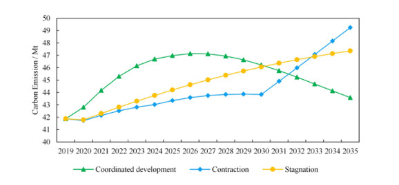
To achieve the goals of carbon peaking and carbon neutrality in Shaanxi, the high energy consuming manufacturing industry (HMI), as an important contributor, is a key link and important channel for energy conservation. In this paper, the logarithmic mean Divisia index (LMDI) method is applied to determine the driving factors of carbon emissions from the aspects of economy, energy and society, and the contribution of these factors was analyzed. Meanwhile, the improved sparrow search algorithm is used to optimize Elman neural network (ENN) to construct a new hybrid prediction model. Finally, three different development scenarios are designed using scenario analysis method to explore the potential of HMI in Shaanxi Province to achieve carbon peak in the future. The results show that: (1) The biggest promoting factor is industrial structure, and the biggest inhibiting factor is energy intensity among the drivers of carbon emissions, which are analyzed effectively in HMI using the LMDI method. (2) Compared with other neural network models, the proposed hybrid prediction model has higher accuracy and better stability in predicting industrial carbon emissions, it is more suitable for simulating the carbon peaking process of HMI. (3) Only in the coordinated development scenario, the HMI in Shaanxi is likely to achieve the carbon peak in 2030, and the carbon emission curve of the other two scenarios has not reached the peak. Then, according to the results of scenario analysis, specific and evaluable suggestions on carbon emission reduction for HMI in Shaanxi are put forward, such as optimizing energy and industrial structure and making full use of innovative resources of Shaanxi characteristic units.
- carbon emission prediction,
- LMDI,
- neural network,
- sparrow search algorithm,
- scenario analysis
Citation: Ke Hou, Jianping Sun, Minggao Dong, He Zhang, Qingqing Li. Simulation of carbon peaking process of high energy consuming manufacturing industry in Shaanxi Province: A hybrid model based on LMDI and TentSSA-ENN[J]. Mathematical Biosciences and Engineering, 2023, 20(10): 18445-18467. doi: 10.3934/mbe.2023819

Related Papers:

Abstract

To achieve the goals of carbon peaking and carbon neutrality in Shaanxi, the high energy consuming manufacturing industry (HMI), as an important contributor, is a key link and important channel for energy conservation. In this paper, the logarithmic mean Divisia index (LMDI) method is applied to determine the driving factors of carbon emissions from the aspects of economy, energy and society, and the contribution of these factors was analyzed. Meanwhile, the improved sparrow search algorithm is used to optimize Elman neural network (ENN) to construct a new hybrid prediction model. Finally, three different development scenarios are designed using scenario analysis method to explore the potential of HMI in Shaanxi Province to achieve carbon peak in the future. The results show that: (1) The biggest promoting factor is industrial structure, and the biggest inhibiting factor is energy intensity among the drivers of carbon emissions, which are analyzed effectively in HMI using the LMDI method. (2) Compared with other neural network models, the proposed hybrid prediction model has higher accuracy and better stability in predicting industrial carbon emissions, it is more suitable for simulating the carbon peaking process of HMI. (3) Only in the coordinated development scenario, the HMI in Shaanxi is likely to achieve the carbon peak in 2030, and the carbon emission curve of the other two scenarios has not reached the peak. Then, according to the results of scenario analysis, specific and evaluable suggestions on carbon emission reduction for HMI in Shaanxi are put forward, such as optimizing energy and industrial structure and making full use of innovative resources of Shaanxi characteristic units.

References

[1]	IPCC, Climate change 2022: Mitigation of climate change, 2022. Available from: https://www.ipcc.ch/report/sixth-assessment-report-working-group-3/
[2]	Xinhua News Agency, Strengthening Action to Address Climate Change: China's National Independent Contribution, 2015. Available from: http://www.gov.cn/xinwen/2015-06/30/content_2887330.htm
[3]	X. Xu, X. Gou, W. Zhang, Y. Zhao, Z. Xu, A bibliometric analysis of carbon neutrality: Research hotspots and future directions, Heliyon, 9 (2023). https://doi.org/10.1016/j.heliyon.2023.e18763 doi: 10.1016/j.heliyon.2023.e18763
[4]	Shaanxi Provincial Development and Reform Commission, Plan for energy conservation and carbon reduction in key areas of high energy consuming industries in Shaanxi Province, 2022. Available from: http://sndrc.Shaanxi.gov.cn/fgyw/tzgg/IjaAVv.htm
[5]	M. Z. Du, F. E. Wu, D. F. Ye, Y. T. Zhao, L. P. Liao, Exploring the effects of energy quota trading policy on carbon emission efficiency: Quasi-experimental evidence from China, Energy Econom., 124 (2023). https://doi.org/10.1016/j.eneco.2023.106791 doi: 10.1016/j.eneco.2023.106791
[6]	Y. Y. Guo, X. J. Gou, Z. S. Xu, M. Skare, Carbon pricing mechanism for the energy industry: A bibliometric study of optimal pricing policies, Acta Montan. Slovaca, 27 (2022), 49–69. https://doi.org/10.46544/AMS.v27i1.05 doi: 10.46544/AMS.v27i1.05
[7]	J. D. Rivera-Niquepa, D. Rojas-Lozano, P. M. De Oliveira-De Jesus, J. M. Yusta, Decomposition analysis of the Aggregate Carbon Intensity (ACI) of the power sector in Colombia-A multi-temporal analysis, Sustainability, 14 (2022). https://doi.org/10.3390/su142013634 doi: 10.3390/su142013634
[8]	Y. Wang, C. Zhang, A. T. Lu, L. Li, Y. M. He, J. J. ToJo, et al., A disaggregated analysis of the environmental Kuznets curve for industrial CO2 emissions in China, Appl. Energy, 190 (2017), 172–180. https://doi.org/10.1016/j.apenergy.2016.12.109 doi: 10.1016/j.apenergy.2016.12.109
[9]	Q. Perrier, C. Guivarch, O. Boucher, Diversity of greenhouse gas emission drivers across European countries since the 2008 crisis, Climate Policy, 19 (2019), 1067–1087. https://doi.org/10.1080/14693062.2019.1625744 doi: 10.1080/14693062.2019.1625744
[10]	D. Zhang, G. Liu, C. Chen, Y. Zhang, Y. Hao, M. Casazza, Medium-to-long-term coupled strategies for energy efficiency and greenhouse gas emissions reduction in Beijing (China), Energy Policy, 127 (2019), 350–360. https://doi.org/10.1016/j.enpol.2018.12.030 doi: 10.1016/j.enpol.2018.12.030
[11]	X. Zou, R. F. Wang, G. H. Hu, Z. Rong, J. X. Li, CO₂ emissions forecast and emissions peak analysis in Shanxi Province, China: An application of the LEAP Model, Sustainability, 14 (2022). https://doi.org/10.3390/su14020637 doi: 10.3390/su14020637
[12]	H. T. Ma, W. Sun, S. J. Wang, L. Kang, Structural contribution and scenario simulation of highway passenger transit carbon emissions in the Beijing-Tianjin-Hebei metropolitan region, China, Resour. Conserv. Recycl., 140 (2019), 209–215. https://doi.org/10.1016/j.resconrec.2018.09.028 doi: 10.1016/j.resconrec.2018.09.028
[13]	H. B. Wang, B. W. Li, M. Q. Khan, Prediction of Shanghai electric power carbon emissions based on improved STIRPAT Model, Sustainability, 14 (2022). https://doi.org/10.3390/su142013068 doi: 10.3390/su142013068
[14]	C. B. Wu, G. H. Huang, B. G. Xin, J. K. Chen, Scenario analysis of carbon emissions' anti-driving effect on Qingdao's energy structure adjustment with an optimization model, Part I: Carbon emissions peak value prediction, J. Cleaner Product., 172 (2018), 466–474. https://doi.org/10.1016/j.jclepro.2017.10.216 doi: 10.1016/j.jclepro.2017.10.216
[15]	X. Q. Liu, Y. M. Ye, D. D. Ge, Z. Wang, B. Liu, Study on the evolution and trends of agricultural carbon emission intensity and agricultural economic development levels-evidence from Jiangxi Province, Sustainability, 14 (2022). https://doi.org/10.3390/su142114265 doi: 10.3390/su142114265
[16]	H. Wang, Z. Zhang, Forecasting Chinese provincial carbon emissions using a novel grey prediction model considering spatial correlation, Expert Syst. Appl., 209 (2022). https://doi.org/10.1016/j.eswa.2022.118261 doi: 10.1016/j.eswa.2022.118261
[17]	Y. S. Huang, L. Shen, H. Liu, Grey relational analysis, principal component analysis and forecasting of carbon emissions based on long short-term memory in China, J. Cleaner Product., 209 (2019), 415–423. https://doi.org/10.1016/j.jclepro.2018.10.128 doi: 10.1016/j.jclepro.2018.10.128
[18]	Z. Zuo, H. Guo, J. Cheng, An LSTM-STRIPAT model analysis of China's 2030 CO₂ emissions peak, Carbon Manag., 11 (2020), 577–592. https://doi.org/10.1080/17583004.2020.1840869 doi: 10.1080/17583004.2020.1840869
[19]	S. AlKheder, A. Almusalam, Forecasting of carbon dioxide emissions from power plants in Kuwait using United States Environmental Protection Agency, Intergovernmental panel on climate change, and machine learning methods, Renewable Energy, 191 (2022), 819–827. https://doi.org/10.1016/j.renene.2022.04.023 doi: 10.1016/j.renene.2022.04.023
[20]	X. Y. Zhou, L. B. Bai, J. Y. Bai, Y. Y. Tian, W. Q. Li, Scenario prediction and critical factors of CO(2)emissions in the Pearl River Delta: A regional imbalanced development perspective, Urban Climate, 44 (2022). https://doi.org/10.1016/j.uclim.2022.101226 doi: 10.1016/j.uclim.2022.101226
[21]	S. Zhang, Z. Huo, C. Zhai, Building carbon emission scenario prediction using STIRPAT and GA-BP neural network model, Sustainability, 14 (2022). https://doi.org/10.3390/su14159369 doi: 10.3390/su14159369
[22]	W. B. Qiao, H. F. Lu, G. F. Zhou, M. Azimi, Q. Yang, W. C. Tian, A hybrid algorithm for carbon dioxide emissions forecasting based on improved lion swarm optimizer, J. Cleaner Product., 244 (2020). https://doi.org/10.1016/j.jclepro.2019.118612 doi: 10.1016/j.jclepro.2019.118612
[23]	F. Kong, J. B. Song, Z. Z. Yang, A novel short-term carbon emission prediction model based on secondary decomposition method and long short-term memory network, Environ. Sci. Pollut. Res., 29 (2022), 64983–64998. https://doi.org/10.1007/s11356-022-20393-w doi: 10.1007/s11356-022-20393-w
[24]	L. Shi, X. Ding, M. Li, Y. Liu, Research on the capability maturity evaluation of intelligent manufacturing based on firefly algorithm, sparrow search algorithm, and BP neural network, Complexity, 2021 (2021). https://doi.org/10.1155/2021/5554215 doi: 10.1155/2021/5554215
[25]	J. Li, W. Wang, G. Chen, Z. Han, Spatiotemporal assessment of landslide susceptibility in Southern Sichuan, China using SA-DBN, PSO-DBN and SSA-DBN models compared with DBN model, Adv. Space Res., 69 (2022), 3071–3087. https://doi.org/10.1016/j.asr.2022.01.043 doi: 10.1016/j.asr.2022.01.043
[26]	W. Guan, Y.-M. Zhu, J.-J. Bao, J. Zhang, Predicting buckling of carbon fiber composite cylindrical shells based on backpropagation neural network improved by sparrow search algorithm, J. Iron Steel Res. Int., (2023). https://doi.org/10.1007/s42243-023-00966-w doi: 10.1007/s42243-023-00966-w
[27]	J. Tang, R. Gong, H. Wang, Y. Liu, Scenario analysis of transportation carbon emissions in China based on machine learning and deep neural network models, Environ. Res. Letters, 18 (2023). https://doi.org/10.1088/1748-9326/acd468 doi: 10.1088/1748-9326/acd468
[28]	J. Hu, J. Bi, H. Liu, Y. Li, S. Ao, Z. Luo, Prediction of resistance spot welding quality based on BPNN optimized by improved sparrow search algorithm, Materials, 15 (2022). https://doi.org/10.3390/ma15207323 doi: 10.3390/ma15207323
[29]	C. Zhao, J. Ma, W. Jia, H. Wang, H. Tian, J. Wang, et al., An apple fungal infection detection model based on BPNN optimized by sparrow search algorithm, Biosensors-Basel, 12 (2022). https://doi.org/10.3390/bios12090692 doi: 10.3390/bios12090692
[30]	M. Yang, Y. S. Liu, Research on the potential for China to achieve carbon neutrality: A hybrid prediction model integrated with elman neural network and sparrow search algorithm, J. Environ. Manag., 329 (2023). https://doi.org/10.1016/j.jenvman.2022.117081 doi: 10.1016/j.jenvman.2022.117081
[31]	Y. Huang, H. Wang, H. Liu, S. Liu, Elman neural network optimized by firefly algorithm for forecasting China's carbon dioxide emissions, Syst. Sci. Control Eng., 7 (2019), 8–15. https://doi.org/10.1080/21642583.2019.1620655 doi: 10.1080/21642583.2019.1620655
[32]	L. G. B. Ruiz, R. Rueda, M. P. Cuellar, M. C. Pegalajar, Energy consumption forecasting based on Elman neural networks with evolutive optimization, Expert Syst. Appl., 92 (2018), 380–389. https://doi.org/10.1016/j.eswa.2017.09.059 doi: 10.1016/j.eswa.2017.09.059
[33]	G. Bedi, G. K. Venayagamoorthy, R. Singh, Development of an IoT-Driven building environment for prediction of electric energy consumption, IEEE Int. Things J., 7 (2020), 4912–4921. https://doi.org/10.1109/jiot.2020.2975847 doi: 10.1109/jiot.2020.2975847
[34]	Y. L. Wang, X. J. Chen, C. L. Li, Y. Yu, G. Zhou, C. Y. Wang, et al., Temperature prediction of lithium-ion battery based on artificial neural network model, Appl. Thermal Eng., 228 (2023). https://doi.org/10.1016/j.applthermaleng.2023.120482
[35]	M. Du, R. Feng, Z. Chen, Blue sky defense in low-carbon pilot cities: A spatial spillover perspective of carbon emission efficiency, Sci. Total Environ., 846 (2022). https://doi.org/10.1016/j.scitotenv.2022.157509
[36]	J. Xue, B. Shen, A novel swarm intelligence optimization approach: Sparrow search algorithm, Syst. Sci. Control Eng., 8 (2020), 22–34. https://doi.org/10.1080/21642583.2019.1708830 doi: 10.1080/21642583.2019.1708830
[37]	J. Feng, J. Zhang, X. Zhu, W. Lian, A novel chaos optimization algorithm, Multi. Tools Appl., 76 (2017), 17405–17436. https://doi.org/10.1007/s11042-016-3907-z doi: 10.1007/s11042-016-3907-z
[38]	Y. Shan, Q. Huang, D. Guan, K. Hubacek, China CO₂ emission accounts 2016–2017, Sci. Data, 7 (2020), 54. https://doi.org/10.1038/s41597-020-0393-y doi: 10.1038/s41597-020-0393-y
[39]	Y. Shan, D. Guan, H. Zheng, J. Ou, Y. Li, J. Meng, et al., China CO₂ emission accounts 1997–2015, Sci. Data, 5 (2018), 170201. https://doi.org/10.1038/sdata.2017.201 doi: 10.1038/sdata.2017.201
[40]	Shaanxi Provincial People's Government, Shaanxi Province " 14th Five-Year Plan" comprehensive work implementation plan for energy conservation and emission reduction, 2022. Available from: http://www.Shaanxi.gov.cn/zfxxgk/fdzdgknr/zcwj/nszfwj/szf/202302/t20230208_2274203.html
[41]	Shaanxi Provincial People's Government, Shaanxi Province industrial carbon peak implementation plan, 2023. Available from: https://www.miit.gov.cn/jgsj/jns/dfdt/art/2023/art_77ae4f2a46414393815d31cab6bb2b8d.html
[42]	Shaanxi Provincial Development and Reform Commission, The 14th Five-Year Plan for the National economic and Social Development of Shaanxi Province and the outline of the long-term goals for 2035, 2021. Available from: http://www.Shaanxi.gov.cn/xw/sxyw/202103/t20210302_2154680.html
[43]	State Council of PRC, National Population Development Plan (2016-2030), 2017. Available from: https://www.gov.cn/gongbao/content/2017/content_5171324.htm
[44]	Shaanxi Provincial People's Government, Shaanxi Provincial Population Development Plan (2016–2030), 2017. Available from: http://www.Shaanxi.gov.cn/zfxxgk/zfgb/2018_3966/d5q_3971/201803/t20180320_1638241_wap.html
[45]	J. J. Tian, X. Q. Song, J. S. Zhang, Prediction on carbon emission peak for typical coal-rich regions in Midwest China, Fresen. Environ. Bull., 31 (2022), 469–479.
[46]	K. Cai, L. F. Wu, Using grey Gompertz model to explore the carbon emission and its peak in 16 provinces of China, Energy Build., 277 (2022). https://doi.org/10.1016/j.enbuild.2022.112545 doi: 10.1016/j.enbuild.2022.112545
[47]	Y. Wu, B. Xu, When will China's carbon emissions peak? Evidence from judgment criteria and emissions reduction paths, Energy Rep., 8 (2022), 8722–8735. https://doi.org/10.1016/j.egyr.2022.06.069 doi: 10.1016/j.egyr.2022.06.069
[48]	C. F. Xu, Y. Zhang, Y. M. A. Yang, H. Y. Gao, Carbon peak scenario simulation of manufacturing carbon emissions in Northeast China: Perspective of structure optimization, Energies, 16 (2023). https://doi.org/10.3390/en16135227 doi: 10.3390/en16135227
[49]	L. L. Sun, H. J. Cui, Q. S. Ge, Will China achieve its 2060 carbon neutral commitment from the provincial perspective?, Adv. Climate Change Res., 13 (2022), 169–178. https://doi.org/10.1016/j.accre.2022.02.002 doi: 10.1016/j.accre.2022.02.002

Reader Comments

Your name:*

Email:*
© 2023 the Author(s), licensee AIMS Press. This is an open access article distributed under the terms of the Creative Commons Attribution License (http://creativecommons.org/licenses/by/4.0)