In positron emission tomography (PET) studies, convolutional neural networks (CNNs) may be applied directly to the reconstructed distribution of radioactive tracers injected into the patient's body, as a pattern recognition tool. Nonetheless, unprocessed PET coincidence data exist in tabular format. This paper develops the transformation of tabular data into $ n $-dimensional matrices, as a preparation stage for classification based on CNNs. This method explicitly introduces a nonlinear transformation at the feature engineering stage and then uses principal component analysis to create the images. We apply the proposed methodology to the classification of simulated PET coincidence events originating from NEMA IEC and anthropomorphic XCAT phantom. Comparative studies of neural network architectures, including multilayer perceptron and convolutional networks, were conducted. The developed method increased the initial number of features from 6 to 209 and gave the best precision results (79.8$ % $) for all tested neural network architectures; it also showed the smallest decrease when changing the test data to another phantom.
Citation: Paweł Konieczka, Lech Raczyński, Wojciech Wiślicki, Oleksandr Fedoruk, Konrad Klimaszewski, Przemysław Kopka, Wojciech Krzemień, Roman Y. Shopa, Jakub Baran, Aurélien Coussat, Neha Chug, Catalina Curceanu, Eryk Czerwiński, Meysam Dadgar, Kamil Dulski, Aleksander Gajos, Beatrix C. Hiesmayr, Krzysztof Kacprzak, Łukasz Kapłon, Grzegorz Korcyl, Tomasz Kozik, Deepak Kumar, Szymon Niedźwiecki, Szymon Parzych, Elena Pérez del Río, Sushil Sharma, Shivani Shivani, Magdalena Skurzok, Ewa Łucja Stępień, Faranak Tayefi, Paweł Moskal. Transformation of PET raw data into images for event classification using convolutional neural networks[J]. Mathematical Biosciences and Engineering, 2023, 20(8): 14938-14958. doi: 10.3934/mbe.2023669
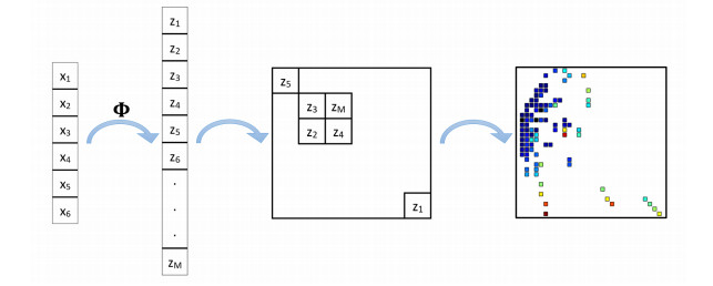
In positron emission tomography (PET) studies, convolutional neural networks (CNNs) may be applied directly to the reconstructed distribution of radioactive tracers injected into the patient's body, as a pattern recognition tool. Nonetheless, unprocessed PET coincidence data exist in tabular format. This paper develops the transformation of tabular data into $ n $-dimensional matrices, as a preparation stage for classification based on CNNs. This method explicitly introduces a nonlinear transformation at the feature engineering stage and then uses principal component analysis to create the images. We apply the proposed methodology to the classification of simulated PET coincidence events originating from NEMA IEC and anthropomorphic XCAT phantom. Comparative studies of neural network architectures, including multilayer perceptron and convolutional networks, were conducted. The developed method increased the initial number of features from 6 to 209 and gave the best precision results (79.8$ % $) for all tested neural network architectures; it also showed the smallest decrease when changing the test data to another phantom.

| [1] |
Y. Lecun, Y. Bengio, G. Hinton, Deep Learning, Nature, 521 (2015), 436—444. https://doi.org/10.1038/nature14539 doi: 10.1038/nature14539

|
| [2] |
M. Z. Alom, T. M. Taha, C. Yakopcic, S. Westberg, P. Sidike, M. S. Nasrin, et al., A state-of-the-art survey on deep learning theory and architectures, Electronics, 8 (2019), 292. https://doi.org/10.3390/electronics8030292 doi: 10.3390/electronics8030292
|
| [3] | A. H. Habibi, H. E. Jahani, Guide to Convolutional Neural Networks: A Practical Application to Traffic-Sign Detection and Classification, Springer International Publishing, 2017. https://doi.org/10.1007/978-3-319-57550-6 |
| [4] | K. He, X. Zhang, S. Ren, J. Sun, Deep Residual Learning for Image Recognition, in Proceedings of the IEEE Conference on Computer Vision and Pattern Recognition, (2016), 770–778. https://doi.org/10.1109/CVPR.2016.90 |
| [5] | J. Redmon, S. Divvala, R. Girshick, A. Farhadi, You only look once: Unfied, real-time object detection, in Proceedings of the IEEE Conference on Computer Vision and Pattern Recognition, (2016), 779–788. https://doi.org/10.1109/CVPR.2015.7298594 |
| [6] | C. Szegedy, W. Liu, Y. Q. Jia, P. Sermanet, S. Reed, D. Anguelov, et al., Going deeper with convolutions, in Proceedings of the IEEE Conference on Computer Vision and Pattern Recognition, (2015), 1–9. https://doi.org/10.48550/arXiv.1409.4842 |
| [7] | C. Szegedy, S. Ioffe, V. Vanhoucke, A. A. Alemi, Inception-v4, inception-ResNet and the impact of residual connections on learning, in Proceedings of the AAAI Conference on Artficial Intelligence, (2017), 4278–4284. https://doi.org/10.48550/arXiv.1602.07261 |
| [8] |
D. S. Kermany, M. Goldbaum, W. J. Cai, C. C. S. Valentim, H. Y. Liang, S. L. Baxter, et al., Identifying medical diagnoses and treatable diseases by image-based deep learning, Cell, 172 (2018), 1122–1131. https://doi.org/10.1016/j.cell.2018.02.010 doi: 10.1016/j.cell.2018.02.010
|
| [9] |
S. Cheng, Y. F. Jin, S. P. Harrison, C. Quilodrán-Casas, L. C. Prentice, Y. K. Guo, et al., Parameter flexible wildfire prediction using machine learning techniques: Forward and inverse modelling, Remote Sens., 14 (2022), 3228. https://doi.org/10.3390/rs14133228 doi: 10.3390/rs14133228
|
| [10] |
Y. Zhuang, S. Cheng, N. Kovalchuk, M. Simmons, O. K. Matar, Y.-K. Guo, et al., Ensemble latent assimilation with deep learning surrogate model: application to drop interaction in a microfluidics device, Lab Chip, 22 (2022), 3187–3202. https://doi.org/10.1039/D2LC00303A doi: 10.1039/D2LC00303A
|
| [11] |
J. L. Humm, A. Rosenfeld, A. Del Guerra, From PET detectors to PET scanners, European J. Nucl. Med. Mol. Imag., 30 (2003), 1574–1597. 10.1007/s00259-003-1266-2 doi: 10.1007/s00259-003-1266-2
|
| [12] | D. L. Bailey, Positron Emission Tomography: Basic Sciences, Springer-Verlag, 2005. https://doi.org/10.1007/b136169 |
| [13] |
A. Alavi, T. J. Werner, E. L. Stępień, P. Moskal, Unparalleled and revolutionary impact of PET imaging on research and day to day practice of medicine, Bio-Algor. Med-Syst., 17 (2021), 203–212. https://doi.org/10.1515/bams-2021-0186 doi: 10.1515/bams-2021-0186
|
| [14] |
E. Berg, S. Cherry, Using convolutional neural networks to estimate time-of-flight from PET detector waveforms, Phys. Med. Biol., 63 (2018), 02LT01. https://doi.org/10.1088/1361-6560/aa9dc5 doi: 10.1088/1361-6560/aa9dc5
|
| [15] | J. Bielecki, Application of the machine learning methods to the multi-photon event classification in the J-PET scanner, M.Sc thesis, Warsaw University of Technology, 2019. Available from: https://pet.ncbj.gov.pl/wp-content/uploads/2019/10/JanBieleckiMasterThesis.pdf |
| [16] |
A. Sharma, E. Vans, D. Shigemizu, K. A. Boroevich, T. Tsunoda, Deepinsight: A methodology to transform a non-image data to an image for convolution neural network architecture, Sci. Rep., 9 (2019), 11399. https://doi.org/10.1038/s41598-019-47765-6 doi: 10.1038/s41598-019-47765-6
|
| [17] |
P. Moskal, Sz. Niedźwiecki, T. Bednarski, E. Czerwiński, Ł. Kapłon, E. Kubicz, et al., Test of a single module of the J-PET scanner based on plastic scintillators, Nucl. Instrum. Meth. Phys. Res. A, 764 (2014), 317–321. https://doi.org/10.1016/j.nima.2014.07.052 doi: 10.1016/j.nima.2014.07.052
|
| [18] |
L. Raczyński, P. Moskal, P. Kowalski, W. Wiślicki, T. Bednarski, P. Białas, et al., Compressive sensing of signals generated in plastic scintillators in a novel J-PET instrument, Nucl. Instrum. Meth. Phys. Res. A, 786 (2015), 105–112. https://doi.org/10.1016/j.nima.2015.03.032 doi: 10.1016/j.nima.2015.03.032
|
| [19] |
P. Moskal, O. Rundel, D. Alfs, T. Bednarski, P. Białas, E. Czerwiński, et al., Time resolution of the plastic scintillator strips with matrix photomultiplier readout for J-PET tomograph, Phys. Med. Biol., 61 (2016), 2025–2047. https://doi.org/10.1088/0031-9155/61/5/2025 doi: 10.1088/0031-9155/61/5/2025
|
| [20] |
S. Niedźwiecki, P. Białas, C. Curceanu, E. Czerwiński, K. Dulski, A. Gajos, et al., J-PET: A new technology for the whole-body PET imaging, Acta Phys. Polon. B, 48 (2017), 1567–1576. https://doi.org/10.5506/APhysPolB.48.1567 doi: 10.5506/APhysPolB.48.1567
|
| [21] |
G. Korcyl, P. Białas, C. Curceanu, E. Czerwiński, K. Dulski, B. Flak, et al., Evaluation of single-chip, real-time tomographic data processing on FPGA—SoC devices, IEEE Trans. Med. Imag., 37 (2018), 2526–2535. https://doi.org/10.1109/TMI.2018.2837741 doi: 10.1109/TMI.2018.2837741
|
| [22] |
P. Moskal, K. Dulski, N. Chug, C. Curceanu, E. Czerwiński, M. Dadgar, et al., Positronium imaging with the novel multiphoton PET scanner, Sci. Adv., 7 (2021), eabh4394. https://doi.org/10.1126/sciadv.abh4394 doi: 10.1126/sciadv.abh4394
|
| [23] |
P. Moskal, A. Gajos, M. Mohammed, J. Chhokar, N. Chug, C. Curceanu, et al., Testing CPT symmetry in ortho-positronium decays with positronium annihilation tomography, Nat. Commun., 12 (2021), 5658. https://doi.org/10.1038/s41467-021-25905-9 doi: 10.1038/s41467-021-25905-9
|
| [24] |
R. D. Badawi, H. C. Shi, P. C. Hu, S. G. Chen, T. Y. Xu, P. M. Price, et al., First human imaging studies with the EXPLORER total-body PET scanner, J. Nuclear Med., 60 (2019), 299–303. https://doi.org/10.2967/jnumed.119.226498 doi: 10.2967/jnumed.119.226498
|
| [25] |
E. N. Holy, A. P. Fan, E. R. Alfaro, E. Fletcher, B. A. Spencer, S. R. Cherry, et al., Non-invasive quantification and SUVR validation of [18F]-florbetaben with total-body EXPLORER PET, Alzheimer's Dement., 18 (2022), e066123. https://doi.org/10.1002/alz.066123 doi: 10.1002/alz.066123
|
| [26] |
S. Vandenberghe, P. Moskal, J. S. Karp, State of the art in total body PET, EJNMMI Phys., 7 (2020), 1–33. https://doi.org/10.1186/s40658-020-00290-2 doi: 10.1186/s40658-020-00290-2
|
| [27] |
A. Rahmim, M. Lenox, A. J. Reader, C. Michel, Z. Burbar, T. J. Ruth, et al., Statistical list-mode image reconstruction for the high resolution research tomograph, Phys. Med. Biol., 49 (2004), 4239–4258. https://doi.org/10.1088/0031-9155/49/18/004 doi: 10.1088/0031-9155/49/18/004
|
| [28] |
R. Accorsi, L.-E. Adam, M. E. Werner, J. S Karp, Optimization of a fully 3D single scatter simulation algorithm for 3D PET, Phys. Med. Biol., 49 (2004), 2577–2598. https://doi.org/10.1088/0031-9155/49/12/008 doi: 10.1088/0031-9155/49/12/008
|
| [29] |
C. C. Watson, Extension of Single Scatter Simulation to Scatter Correction of Time-of-Flight PET, IEEE Trans. Nucl. Sci., 54 (2007), 1679–1686. https://doi.org/10.1109/TNS.2007.901227 doi: 10.1109/TNS.2007.901227
|
| [30] | L. J. Maaten, G. Hinton, Visualizing High-Dimesional Data using t-SNE, J. Mach. Learn. Research, 9 (2008), 2579–2605. Available from: https://www.jmlr.org/papers/volume9/vandermaaten08a/vandermaaten08a.pdf. |
| [31] |
B. Scholkopf, S. A. Bernhard, K. R. Muller, Nonlinear component analysis as a kernel eigenvalue problem, Neural Comput., 10 (1998), 1299–1319. https://doi.org/10.1162/089976698300017467 doi: 10.1162/089976698300017467
|
| [32] | M. A. Aizerman, E. M. Braverman, L. I. Rozonoer, Theoretical foundations of the potential function method in pattern recognition learning, Autom. Remote Control, 25 (1964), 821–837. Available from: https://cs.uwaterloo.ca/y328yu/classics/kernel.pdf |
| [33] | V. Vapnik, The Nature of Statistical Learning Theory, Springer-Verlag, 1995. https://doi.org/10.1007/978-1-4757-2440-0 |
| [34] | V. Vapnik, Statistical Learning Theory, Wiley, 1998. Available from: https://www.wiley.com/en-ie/Statistical+Learning+Theory-p-9780471030034 |
| [35] |
J. Mockus, Application of Bayesian approach to numerical methods of global and stochastic optimization, J. Global Optim., 4 (1994), 347–365. https://doi.org/10.1007/BF01099263 doi: 10.1007/BF01099263
|
| [36] |
S. Jan, G. Santin, D. Strul, S. Staelens, K. Assié, D. Autret, et al., GATE: A simulation toolkit for PET and SPECT, Phys. Med. Biol., 49 (2004), 454-4562. https://doi.org/10.1088/0031-9155/49/19/007 doi: 10.1088/0031-9155/49/19/007
|
| [37] |
D. Sarrut, M. Bała, M. Bardiès, J. Bert, M. Chauvin, K. Chatzipapas, et al., Advanced Monte Carlo simulations of emission tomography imaging systems with GATE, Phys. Med. Biol., 66 (2021), 10TR03. https://doi.org/10.1088/1361-6560/abf276 doi: 10.1088/1361-6560/abf276
|
| [38] | J. Baran, W. Krzemien, L. Raczyński, M. Bała, A. Coussat, S. Parzych, et al., Realistic Total-Body J-PET Geometry Optimization–Monte Carlo Study, preprint arXiv e-prints, (2022), arXiv: 2212.02285. https://doi.org/10.48550/arXiv.2212.02285 |
| [39] | NEMA Standards Publication NU 2-2007: Performance measurements of Positron Emission Tomographs, Nat. Elect. Manuf. Assoc., (2007). Available from: https://psec.uchicago.edu/library/applications/PET/chien_min_NEMA_NU2_2007.pdf |
| [40] |
W. P. Segars, G. Sturgeon, S. Mendonca, J. Grimes, B. M. W. Tsui, 4D XCAT phantom for multimodality imaging research, Med. Phys., 37 (2010), 4902–4915. https://doi.org/10.1118/1.3480985 doi: 10.1118/1.3480985
|
| [41] |
P. Kowalski, W. Wi'slicki, L. Raczy'nski, D. Alfs, T. Bednarski, P. Bialas, et al., Scatter fraction of the J-PET tomography scanner, Acta Phys. Pol. B, 47 (2016), 549–560. https://doi.org/10.5506/APhysPolB.47.549 doi: 10.5506/APhysPolB.47.549
|
| [42] |
M. Pawlik-Niedźwiecka, S. Niedźwiecki, D. Alfs, P. Bialas, C. Curceanu, E. Czerwiński, et al., Preliminary studies of J-PET detector spatial resolution, Acta Phys. Polon. A, 132 (2017), 1645–1648. https://doi.org/10.12693/APhysPolA.132.1645 doi: 10.12693/APhysPolA.132.1645
|
| [43] |
P. Moskal, P. Kowalski, R. Y. Shopa, L. Raczyński, J. Baran, N. Chug, et al., Simulating NEMA characteristics of the modular total-body J-PET scanner - an economic total-body PET from plastic scintillators, Phys. Med. Biol., 66 (2021), 175015. https://doi.org/10.1088/1361-6560/ac16bd doi: 10.1088/1361-6560/ac16bd
|
| [44] |
F. Murtagh, Multilayer perceptrons for classification and regression, Neurocomputing, 2 (1991), 183–197. https://doi.org/10.1016/0925-2312(91)90023-5 doi: 10.1016/0925-2312(91)90023-5
|
| [45] |
H. Ramchoun, M. A. Janati Idrissi, Y. Ghanou, M. Ettaouil, Multilayer perceptron: Architecture optimization and training, Int. J. Interact. Multim. Artif. Intell., 4 (2016), 26–30. https://doi.org/10.9781/ijimai.2016.415 doi: 10.9781/ijimai.2016.415
|
| [46] | A. Landi, P. Piaggi, M. Laurino, D. Menicucci, Artificial neural networks for nonlinear regression and classification, in 2010 10th International Conference on Intelligent Systems Design and Applications, (2010), 115–120. https://doi.org/10.1109/ISDA.2010.5687280 |


Figures(11) / Tables(4)

Paweł Konieczka, Lech Raczyński, Wojciech Wiślicki, Oleksandr Fedoruk, Konrad Klimaszewski, Przemysław Kopka, Wojciech Krzemień, Roman Y. Shopa, Jakub Baran, Aurélien Coussat, Neha Chug, Catalina Curceanu, Eryk Czerwiński, Meysam Dadgar, Kamil Dulski, Aleksander Gajos, Beatrix C. Hiesmayr, Krzysztof Kacprzak, Łukasz Kapłon, Grzegorz Korcyl, Tomasz Kozik, Deepak Kumar, Szymon Niedźwiecki, Szymon Parzych, Elena Pérez del Río, Sushil Sharma, Shivani Shivani, Magdalena Skurzok, Ewa Łucja Stępień, Faranak Tayefi, Paweł Moskal. Transformation of PET raw data into images for event classification using convolutional neural networks[J]. Mathematical Biosciences and Engineering, 2023, 20(8): 14938-14958. doi: 10.3934/mbe.2023669


 DownLoad: