Methamphetamine (meth) addiction is a significant social and public health problem worldwide. The relapse rate of meth abstainers is significantly high, but the underlying physiological mechanisms are unclear. Therefore, in this study, we performed resting-state functional magnetic resonance imaging (rs-fMRI) analysis to detect differences in the spontaneous neural activity between the meth abstainers and the healthy controls, and identify the physiological mechanisms underlying the high relapse rate among the meth abstainers. The fluctuations and time variations in the blood oxygenation level-dependent (BOLD) signal of the local brain activity was analyzed from the pre-processed rs-fMRI data of 11 meth abstainers and 11 healthy controls and estimated the amplitude of low-frequency fluctuations (ALFF) and the dynamic ALFF (dALFF). In comparison with the healthy controls, meth abstainers showed higher ALFF in the anterior central gyrus, posterior central gyrus, trigonal-inferior frontal gyrus, middle temporal gyrus, dorsolateral superior frontal gyrus, and the insula, and reduced ALFF in the paracentral lobule and middle occipital gyrus. Furthermore, the meth abstainers showed significantly reduced dALFF in the supplementary motor area, orbital inferior frontal gyrus, middle frontal gyrus, medial superior frontal gyrus, middle occipital gyrus, insula, middle temporal gyrus, anterior central gyrus, and the cerebellum compared to the healthy controls ($ P < 0.05 $). These data showed abnormal spontaneous neural activity in several brain regions related to the cognitive, executive, and other social functions in the meth abstainers and potentially represent the underlying physiological mechanisms that are responsible for the high relapse rate. In conclusion, a combination of ALFF and dALFF analytical methods can be used to estimate abnormal spontaneous brain activity in the meth abstainers and make a more reasonable explanation for the high relapse rate of meth abstainers.
Citation: Guixiang Liang, Xiang Li, Hang Yuan, Min Sun, Sijun Qin, Benzheng Wei. Abnormal static and dynamic amplitude of low-frequency fluctuations in multiple brain regions of methamphetamine abstainers[J]. Mathematical Biosciences and Engineering, 2023, 20(7): 13318-13333. doi: 10.3934/mbe.2023593
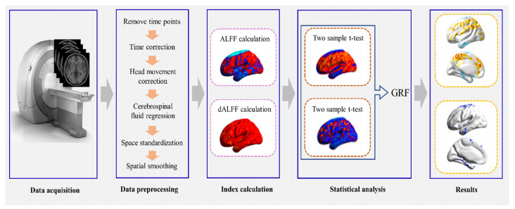
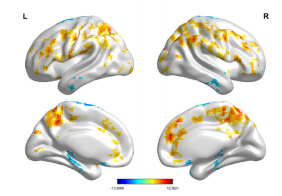
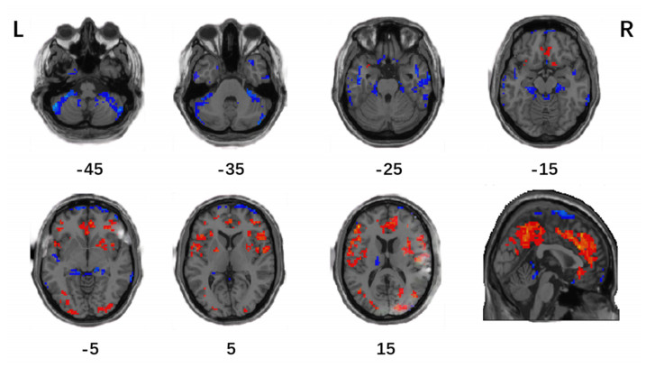
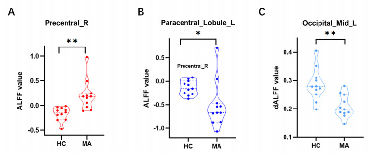
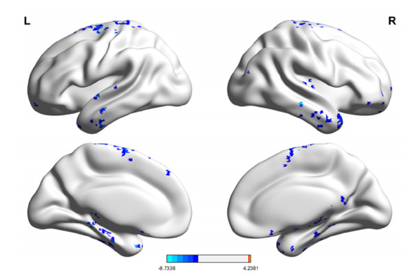
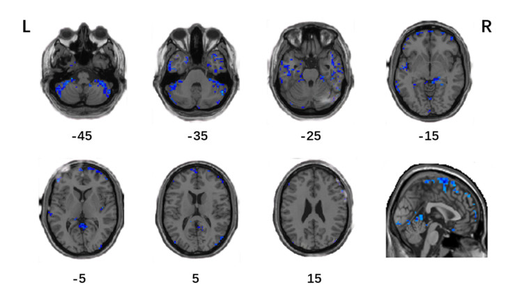
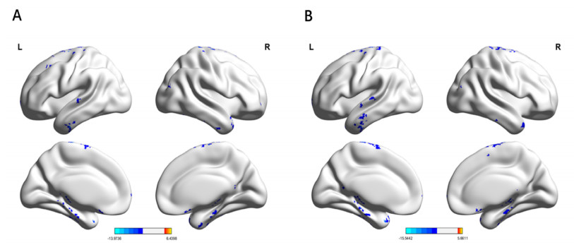
Methamphetamine (meth) addiction is a significant social and public health problem worldwide. The relapse rate of meth abstainers is significantly high, but the underlying physiological mechanisms are unclear. Therefore, in this study, we performed resting-state functional magnetic resonance imaging (rs-fMRI) analysis to detect differences in the spontaneous neural activity between the meth abstainers and the healthy controls, and identify the physiological mechanisms underlying the high relapse rate among the meth abstainers. The fluctuations and time variations in the blood oxygenation level-dependent (BOLD) signal of the local brain activity was analyzed from the pre-processed rs-fMRI data of 11 meth abstainers and 11 healthy controls and estimated the amplitude of low-frequency fluctuations (ALFF) and the dynamic ALFF (dALFF). In comparison with the healthy controls, meth abstainers showed higher ALFF in the anterior central gyrus, posterior central gyrus, trigonal-inferior frontal gyrus, middle temporal gyrus, dorsolateral superior frontal gyrus, and the insula, and reduced ALFF in the paracentral lobule and middle occipital gyrus. Furthermore, the meth abstainers showed significantly reduced dALFF in the supplementary motor area, orbital inferior frontal gyrus, middle frontal gyrus, medial superior frontal gyrus, middle occipital gyrus, insula, middle temporal gyrus, anterior central gyrus, and the cerebellum compared to the healthy controls ($ P < 0.05 $). These data showed abnormal spontaneous neural activity in several brain regions related to the cognitive, executive, and other social functions in the meth abstainers and potentially represent the underlying physiological mechanisms that are responsible for the high relapse rate. In conclusion, a combination of ALFF and dALFF analytical methods can be used to estimate abnormal spontaneous brain activity in the meth abstainers and make a more reasonable explanation for the high relapse rate of meth abstainers.

| [1] |
B. R. Lee, S. J. Sung, K. H. Hur, S. E. Kim, S. X. Ma, S. K. Kim, et al., Korean Red Ginseng inhibits methamphetamine addictive behaviors by regulating dopaminergic and NMDAergic system in rodents, J. Ginseng Res., 46 (2022), 147–155. https://doi.org/10.1016/j.jgr.2021.05.007 doi: 10.1016/j.jgr.2021.05.007

|
| [2] |
D. M. Stoneberg, R. K. Shukla, M. B. Magness, Global methamphetamine trends: an evolving problem, Int. Crim. Justice Rev., 28 (2018), 136–161. https://doi.org/10.1177/1057567717730104 doi: 10.1177/1057567717730104
|
| [3] |
L. Xu, L. Li, Q. Chen, Y. Huang, X. Chen, D. Qiao, The role of non-coding RNAs in methamphetamine-induced neurotoxicity, Cell. Mol. Neurobiol., 2023 (2023), 1–22. https://doi.org/10.1007/s10571-023-01323-x doi: 10.1007/s10571-023-01323-x
|
| [4] |
C. J. Kuo, Y. T. Liao, W. J. Chen, S. Y. Tsai, S. K. Lin, C. C. Chen, Causes of death of patients with methamphetamine dependence: a record‐linkage study, Drug Alcohol. Rev., 30 (2011), 621–628. https://doi.org/10.1111/j.1465-3362.2010.00255.x doi: 10.1111/j.1465-3362.2010.00255.x
|
| [5] | World Drug Report 2022, UN Office on Drugs and Crime, 2022. Available from: https://www.unodc.org/unodc/data-and-analysis/world-drug-report-2022.html. |
| [6] |
P. Jiang, J. Y. Sun, X. B. Zhou, L. Lu, L. Li, X. Q. Huang, et al., Functional connectivity abnormalities underlying mood disturbances in male abstinent methamphetamine abusers, Hum. Brain Mapp., 42 (2021), 3366–3378. https://doi.org/10.1002/hbm.25439 doi: 10.1002/hbm.25439
|
| [7] |
P. J. McCarty, A. R. Pines, B. L. Sussman, S. N. Wyckoff, A. Jensen, R. Bunch, et al., Resting state functional magnetic resonance imaging elucidates neurotransmitter deficiency in autism spectrum disorder, J. Pers. Med., 11 (2021), https://doi.org/10.3390/jpm11100969 doi: 10.3390/jpm11100969
|
| [8] |
Y. Y. Du, W. H. Yang, J. Zhang, J. Liu, Changes in ALFF and ReHo values in methamphetamine abstinent individuals based on the Harvard-Oxford atlas: A longitudinal resting-state fMRI study, Addict. Biol., 27 (2022), e13080. https://doi.org/10.1111/adb.13080 doi: 10.1111/adb.13080
|
| [9] |
M. Q. Gong, Y. X. Shen, W. B. Liang, Z. Zhang, C. X. He, M. W. Lou, et al., Impairments in the default mode and executive networks in methamphetamine usersduring short-term abstinence, Int. J. Gen. Med., 15 (2022), 6073–6084. https://doi.org/10.2147/ijgm.S369571 doi: 10.2147/ijgm.S369571
|
| [10] |
O. Sporns, The non-random brain: efficiency, economy, and complex dynamics, Front. Comput. Neurosci., 5 (2011), 5. https://doi.org/10.3389/fncom.2011.00005 doi: 10.3389/fncom.2011.00005
|
| [11] |
W. Liao, G. R. Wu, Q. Xu, G. J. Ji, Z. Q. Zhang, Y. F. Zang, et al., DynamicBC: a MATLAB toolbox for dynamic brain connectome analysis, Brain Connect., 4 (2014), 780–790. https://doi.org/10.1089/brain.2014.0253 doi: 10.1089/brain.2014.0253
|
| [12] |
Q. Cui, W. Sheng, Y. Y. Chen, Y. J. Pang, F. M. Lu, Q. Tang, et al., Dynamic changes of amplitude of low-frequency fluctuations in patients with generalized anxiety disorder, Hum. Brain Mapp., 41 (2020), 1667–1676. https://doi.org/10.1002/hbm.24902 doi: 10.1002/hbm.24902
|
| [13] |
J. Li, X. J. Duan, Q. Cui, H. F. Chen, W. Liao, More than just statics: temporal dynamics of intrinsic brain activity predicts the suicidal ideation in depressed patients, Psychol. Med., 49 (2019), 852–860. https://doi.org/10.1017/s0033291718001502 doi: 10.1017/s0033291718001502
|
| [14] |
Z. Fu, A. Iraji, J. A. Turner, J. Sui, R. Miller, G. D. Pearlson, et al., Dynamic state with covarying brain activity-connectivity: On the pathophysiology of schizophrenia, Neuroimage, 224 (2021), 117385. https://doi.org/10.1016/j.neuroimage.2020.117385 doi: 10.1016/j.neuroimage.2020.117385
|
| [15] |
C. G. Yan, X. D. Wang, X. N. Zuo, Y. F. Zang, DPABI: data processing & analysis for (resting-state) brain imaging, Neuroinformatics, 14 (2016), 339–351. https://doi.org/10.1007/s12021-016-9299-4 doi: 10.1007/s12021-016-9299-4
|
| [16] |
J. J. Wang, X. Chen, S. K. Sah, C. Zeng, Y. M. Li, N. Li, et al., Amplitude of low-frequency fluctuation (ALFF) and fractional ALFF in migraine patients: a resting-state functional MRI study, Clin. Radiol., 71 (2016), 558–564. https://doi.org/10.1016/j.crad.2016.03.004 doi: 10.1016/j.crad.2016.03.004
|
| [17] |
H. Yuan, X. H. Yu, X. Li, S. J. Qin, G. X. Liang, T. Y. Bai, et al., Research on resting spontaneous brain activity and functional connectivity of acupuncture at uterine acupoints, Digital Chin. Med., 5 (2022), 59–67. https://doi.org/10.1016/j.dcmed.2022.03.006 doi: 10.1016/j.dcmed.2022.03.006
|
| [18] |
R. Li, W. Liao, Y. Y. Yu, H. Chen, X. N. Guo, Y. L. Tang, et al., Differential patterns of dynamic functional connectivity variability of striato-cortical circuitry in children with benign epilepsy with centrotemporal spikes, Hum. Brain Mapp., 39 (2018), 1207–1217. https://doi.org/10.1002/hbm.23910 doi: 10.1002/hbm.23910
|
| [19] |
Q. Li, X. H. Cao, S. Liu, Z. X. Li, Y. F. Wang, L. Cheng, et al., Dynamic alterations of amplitude of low-frequency fluctuations in patients with drug-naive first-episode early onset schizophrenia, Front. Neurosci., 14 (2020), 901. https://doi.org/10.3389/fnins.2020.00901 doi: 10.3389/fnins.2020.00901
|
| [20] |
W. Liao, J. Li, G. J. Ji, G. R. Wu, Z. Long, Q. Xu, et al., Endless fluctuations: temporal dynamics of the amplitude of low frequency fluctuations, IEEE Trans. Med. Imaging, 38 (2019), 2523–2532. https://doi.org/10.1109/TMI.2019.2904555 doi: 10.1109/TMI.2019.2904555
|
| [21] | A. Ardila, Executive functions brain functional system, in Dysexecutive syndromes: Clinical and experimental perspectives, Springer Press, (2019), 29–41. https://doi.org/10.1007/978-3-030-25077-5_2 |
| [22] |
M. Gong, W. Liang, C. He, Y. Shen, Z. Zhang, M. Lou, et al., Neuroimaging mechanisms in short-term heroin-and methamphetamine-abstinent users: Similarities and differences, Neurosci. Lett., 796 (2023), 137057. https://doi.org/10.1016/j.neulet.2023.137057 doi: 10.1016/j.neulet.2023.137057
|
| [23] | J. G. Scott, M. R. Schoenberg, Frontal lobe/executive functioning, in The little black book of neuropsychology: A syndrome-based approach, Springer Press, (2010) 219–248. https://doi.org/10.1007/978-0-387-76978-3_10 |
| [24] |
W. Sato, M. Toichi, S. Uono, T. Kochiyama, Impaired social brain network for processing dynamic facial expressions in autism spectrum disorders, BMC Neurosci., 13 (2012), 1–17. https://doi.org/10.1186/1471-2202-13-99 doi: 10.1186/1471-2202-13-99
|
| [25] |
W. Xie, J. I. Chapeton, S. Bhasin, C. Zawora, J. H. Wittig Jr, S. K. Inati, et al., The medial temporal lobe supports the quality of visual short-term memory representation, Nat. Hum. Behav., 7 (2023), 627–641. https://doi.org/10.1038/s41562-023-01529-5 doi: 10.1038/s41562-023-01529-5
|
| [26] |
A. Avena-Koenigsberger, B. Misic, O. Sporns, Communication dynamics in complex brain networks, Nat. Rev. Neurosci., 19 (2018), 17–33. https://doi.org/10.1038/nrn.2017.149 doi: 10.1038/nrn.2017.149
|
| [27] |
Y. Li, L. Liu, E. Wang, H. Zhang, S. Dou, L. Tong, et al., Abnormal neural network of primary insomnia: evidence from spatial working memory task fMRI, Eur. Neurol., 75 (2016), 48–57. https://doi.org/10.1159/000443372 doi: 10.1159/000443372
|
| [28] |
T. P. Zanto, A. Gazzaley, Fronto-parietal network: flexible hub of cognitive control, Trends Cognit. Sci., 17 (2013), 602–603. https://doi.org/10.1016/j.tics.2013.10.001 doi: 10.1016/j.tics.2013.10.001
|
| [29] |
D. Vuletic, P. Dupont, F. Robertson, J. Warwick, J. R. Zeevaart, D. J. Stein, Methamphetamine dependence with and without psychotic symptoms: A multi-modal brain imaging study, Neuroimage Clin., 20 (2018), 1157–1162. https://doi.org/10.1016/j.nicl.2018.10.023 doi: 10.1016/j.nicl.2018.10.023
|
| [30] |
U. Wolf, M. J. Rapoport, T. A. Schweizer, Evaluating the affective component of the cerebellar cognitive affective syndrome, J. Neuropsychiatry Clin. Neurosci., 21 (2009), 245–253. https://doi.org/10.1176/jnp.2009.21.3.245 doi: 10.1176/jnp.2009.21.3.245
|
| [31] |
E. A. Moulton, I. Elman, L. R. Becerra, R. Z. Goldstein, D. Borsook, The cerebellum and addiction: insights gained from neuroimaging research, Addict. Biol., 19 (2014), 317–331. https://doi.org/10.1111/adb.12101 doi: 10.1111/adb.12101
|
| [32] |
X. T. Li, H. Su, N. Zhong, T. Z. Chen, J. Du, K. Xiao, et al., Aberrant resting-state cerebellar-cerebral functional connectivity in methamphetamine-dependent individuals after six months abstinence, Front. Psychiatry, 11 (2020), 191. https://doi.org/10.3389/fpsyt.2020.00191 doi: 10.3389/fpsyt.2020.00191
|
| [33] |
M. Malina, S. Keedy, J. Weafer, K. Van Hedger, H. de Wit, Effects of methamphetamine on within-and between-network connectivity in healthy adults, Cereb. Cortex, 2 (2021), tgab063. https://doi.org/10.1093/texcom/tgab063 doi: 10.1093/texcom/tgab063
|
| [34] | A. Sathyanesan, J. Zhou, J. Scafidi, D. H. Heck, R. V. Sillitoe, V. Gallo, Emerging connections between cerebellar development, behaviour and complex brain disorders, Nat. Rev. Neurosci., 20 (2019), 298–313. https://doi.org/10.1038/s41583-019-0152-2 |
| [35] | E. A. Evans, C. E. Grella, D. M. Upchurch, Gender differences in the effects of childhood adversity on alcohol, drug, and polysubstance-related disorders, Social Psychiatry Psychiatr. Epidemiol., 52 (2017), 901–912. https://doi.org/10.1007/s00127-017-1355-3 |
| [36] |
K. Ratheesh, L. Seah, V. Murukeshan, Spectral phase-based automatic calibration scheme for swept source-based optical coherence tomography systems, Phys. Med. Biol., 61 (2016), 7652. https://doi.org/10.1088/0031-9155/61/21/7652 doi: 10.1088/0031-9155/61/21/7652
|
| [37] |
R. K. Meleppat, K. E. Ronning, S. J. Karlen, M. E. Burns, E. N. Pugh, R. J. Zawadzki, In vivo multimodal retinal imaging of disease-related pigmentary changes in retinal pigment epithelium, Sci. Rep., 11 (2021), 1–14. https://doi.org/10.1038/s41598-021-95320-z doi: 10.1038/s41598-021-95320-z
|
| [38] |
R. K. Meleppat, C. R. Fortenbach, Y. Jian, E. S. Martinez, K. Wagner, B. S. Modjtahedi, et al., In vivo imaging of retinal and choroidal morphology and vascular plexuses of vertebrates using swept-source optical coherence tomography, Transl. Vision Sci. Technol., 11 (2022), 11. https://doi.org/10.1167/tvst.11.8.11 doi: 10.1167/tvst.11.8.11
|
| [39] |
R. K. Meleppat, C. Shearwood, S. L. Keey, M. V. Matham, Quantitative optical coherence microscopy for the in situ investigation of the biofilm, J. Biomed. Opt., 21 (2016), 127002–127002. http://dx.doi.org/10.1117/1.JBO.21.12.127002 doi: 10.1117/1.JBO.21.12.127002
|
| [40] | W. Abada, A. Bouramoul, Using machinelearning techniques to predict people at-risk for drug addiction: A Bayesian-Based Model, in 2022 4th International Conference on Pattern Analysis and Intelligent Systems (PAIS), IEEE, (2022), 1–7. https://doi.org/10.1109/PAIS56586.2022.9946914 |
| [41] |
H. Chen, C. Li, G. Wang, X. Li, M. M. Rahaman, H. Sun, et al., GasHis-Transformer: A multi-scale visual transformer approach for gastric histopathological image detection, Pattern Recognit., 130 (2022), 108827. https://doi.org/10.1016/j.patcog.2022.108827 doi: 10.1016/j.patcog.2022.108827
|
Figures(7) / Tables(3)

Guixiang Liang, Xiang Li, Hang Yuan, Min Sun, Sijun Qin, Benzheng Wei. Abnormal static and dynamic amplitude of low-frequency fluctuations in multiple brain regions of methamphetamine abstainers[J]. Mathematical Biosciences and Engineering, 2023, 20(7): 13318-13333. doi: 10.3934/mbe.2023593


 DownLoad: