Realistic simulation of time-course measurements in systems biology

Janine Egert; Clemens Kreutz; Janine Egert; Clemens Kreutz

doi:10.3934/mbe.2023467

Mathematical Biosciences and Engineering

2023, Volume 20, Issue 6: 10570-10589. doi: 10.3934/mbe.2023467

Previous Article Next Article

Research article Special Issues

Realistic simulation of time-course measurements in systems biology

Janine Egert ^1,2,
Clemens Kreutz ^{1,2,3
,
,}

1.
Institute of Medical Biometry and Statistics (IMBI), Faculty of Medicine and Medical Center – University of Freiburg, Stefan-Meier-Str. 26, 79104 Freiburg, Germany
2.
Centre for Integrative Biological Signalling Studies CIBSS, University of Freiburg, 79104 Freiburg, Germany
3.
Center for Data Analysis and Modelling (FDM), University of Freiburg, 79104 Freiburg, Germany

Academic Editor: Zhuolin Qu

Received: 28 December 2022 Revised: 29 March 2023 Accepted: 30 March 2023 Published: 11 April 2023

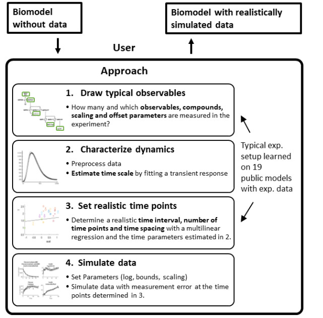
In systems biology, the analysis of complex nonlinear systems faces many methodological challenges. For the evaluation and comparison of the performances of novel and competing computational methods, one major bottleneck is the availability of realistic test problems. We present an approach for performing realistic simulation studies for analyses of time course data as they are typically measured in systems biology. Since the design of experiments in practice depends on the process of interest, our approach considers the size and the dynamics of the mathematical model which is intended to be used for the simulation study. To this end, we used 19 published systems biology models with experimental data and evaluated the relationship between model features (e.g., the size and the dynamics) and features of the measurements such as the number and type of observed quantities, the number and the selection of measurement times, and the magnitude of measurement errors. Based on these typical relationships, our novel approach enables suggestions of realistic simulation study designs in the systems biology context and the realistic generation of simulated data for any dynamic model. The approach is demonstrated on three models in detail and its performance is validated on nine models by comparing ODE integration, parameter optimization, and parameter identifiability. The presented approach enables more realistic and less biased benchmark studies and thereby constitutes an important tool for the development of novel methods for dynamic modeling.
- systems biology,
- simulation,
- method evaluation,
- benchmark,
- model dynamics
Citation: Janine Egert, Clemens Kreutz. Realistic simulation of time-course measurements in systems biology[J]. Mathematical Biosciences and Engineering, 2023, 20(6): 10570-10589. doi: 10.3934/mbe.2023467

Related Papers:

Abstract

In systems biology, the analysis of complex nonlinear systems faces many methodological challenges. For the evaluation and comparison of the performances of novel and competing computational methods, one major bottleneck is the availability of realistic test problems. We present an approach for performing realistic simulation studies for analyses of time course data as they are typically measured in systems biology. Since the design of experiments in practice depends on the process of interest, our approach considers the size and the dynamics of the mathematical model which is intended to be used for the simulation study. To this end, we used 19 published systems biology models with experimental data and evaluated the relationship between model features (e.g., the size and the dynamics) and features of the measurements such as the number and type of observed quantities, the number and the selection of measurement times, and the magnitude of measurement errors. Based on these typical relationships, our novel approach enables suggestions of realistic simulation study designs in the systems biology context and the realistic generation of simulated data for any dynamic model. The approach is demonstrated on three models in detail and its performance is validated on nine models by comparing ODE integration, parameter optimization, and parameter identifiability. The presented approach enables more realistic and less biased benchmark studies and thereby constitutes an important tool for the development of novel methods for dynamic modeling.

References

[1]	A. Degasperi, D. Fey, B. N. Kholodenko, Performance of objective functions and optimisation procedures for parameter estimation in system biology models, npj Syst. Biol. Appl., 3 (2017). https://doi.org/10.1038/s41540-017-0023-2 doi: 10.1038/s41540-017-0023-2
[2]	C. Kreutz, New Concepts for Evaluating the Performance of Computational Methods, IFAC-PapersOnLine, 49 (2016), 63–70. https://doi.org/10.1016/j.ifacol.2016.12.104 doi: 10.1016/j.ifacol.2016.12.104
[3]	R. J. Prill, D. Marbach, J. Saez-Rodriguez, P. K. Sorger, L. G. Alexopoulos, X. Xue, et al., Towards a Rigorous Assessment of Systems Biology Models: The DREAM3 Challenges, PLoS ONE, 5 (2010), e9202. https://doi.org/10.1371/journal.pone.0009202 doi: 10.1371/journal.pone.0009202
[4]	A. Raue, M. Schilling, J. Bachmann, A. Matteson, M. Schelke, D. Kaschek, et al., Lessons Learned from Quantitative Dynamical Modeling in Systems Biology, PLoS ONE, 8 (2013), e74335. https://doi.org/10.1371/journal.pone.0074335 doi: 10.1371/journal.pone.0074335
[5]	P. Städter, Y. Schälte, L. Schmiester, J. Hasenauer, P. L. Stapor, Benchmarking of numerical integration methods for ODE models of biological systems, Sci. Rep., 11 (2021), 2969. https://doi.org/10.1038/s41598-021-82196-2 doi: 10.1038/s41598-021-82196-2
[6]	P. Stapor, F. Fröhlich, J. Hasenauer, Optimization and profile calculation of ODE models using second order adjoint sensitivity analysis, Bioinformatics, 34 (2018), i151–i159. https://doi.org/10.1093/bioinformatics/bty230 doi: 10.1093/bioinformatics/bty230
[7]	A. F. Villaverde, F. Fröhlich, D. Weindl, J. Hasenauer, J. R. Banga, Benchmarking optimization methods for parameter estimation in large kinetic models, Bioinformatics, 35 (2018), 830–838. https://doi.org/10.1093/bioinformatics/bty736 doi: 10.1093/bioinformatics/bty736
[8]	N. Le Novere, B. Bornstein, A. Broicher, M. Courtot, M. Donizelli, H. Dharuri, et al., BioModels Database: a free, centralized database of curated, published, quantitative kinetic models of biochemical and cellular systems, Nucleic Acids Res., 34 (2006), D689–D691. https://doi.org/10.1093/nar/gkj092 doi: 10.1093/nar/gkj092
[9]	M. Hucka, A. Finney, H. M. Sauro, H. Bolouri, J. C. Doyle, H. Kitano, et al., The systems biology markup language (SBML): a medium for representation and exchange of biochemical network models, Bioinformatics, 19 (2003), 524–531. https://doi.org/10.1093/bioinformatics/btg015 doi: 10.1093/bioinformatics/btg015
[10]	H. Hass, C. Loos, E. Raimundez-Alvarez, J. Timmer, J. Hasenauer, C. Kreutz, Benchmark problems for dynamic modeling of intracellular processes, Bioinformatics, 35 (2019), 3073–3082. https://doi.org/10.1093/bioinformatics/btz020 doi: 10.1093/bioinformatics/btz020
[11]	A. F. Villaverde, D. Henriques, K. Smallbone, S. Bongard, J. Schmid, D. Cicin-Sain, et al., BioPreDyn-bench: a suite of benchmark problems for dynamic modelling in systems biology, BMC Syst. Biol., 9 (2015). https://doi.org/10.1186/s12918-015-0144-4 doi: 10.1186/s12918-015-0144-4
[12]	L. Schmiester, Y. Schälte, F. T. Bergmann, T. Camba, E. Dudkin, J. Egert, et al., PEtab–Interoperable specification of parameter estimation problems in systems biology, PLoS Comput. Biol., 17 (2021), e1008646. https://doi.org/10.1371/journal.pcbi.1008646 doi: 10.1371/journal.pcbi.1008646
[13]	C. Kreutz, A New Approximation Approach for Transient Differential Equation Models, Front. Phys., 8 (2020), 1–14. https://doi.org/10.3389/fphy.2020.00070 doi: 10.3389/fphy.2020.00070
[14]	A. Raue, B. Steiert, M. Schelker, C. Kreutz, T. Maiwald, H. Hass, et al., Data2Dynamics: a modeling environment tailored to parameter estimation in dynamical systems, Bioinformatics, 31 (2015), 3558–3560. https://doi.org/10.1093/bioinformatics/btv405 doi: 10.1093/bioinformatics/btv405
[15]	O. Alkan, B. Schoeberl, M. Shah, A. Koshkaryev, T. Heinemann, D. C. Drummond, et al., Modeling chemotherapy-induced stress to identify rational combination therapies in the DNA damage response pathway, Sci. Signal., 11 (2018), eaat0229. https://doi.org/10.1126/scisignal.aat0229 doi: 10.1126/scisignal.aat0229
[16]	J. Bachman, A. Raue, M. Schilling, M. E. Böhm, C. Kreutz, D. Kaschek, et al., Division of labor by dual feedback regulators controls JAK2/STAT5 signaling over broad ligand range, Mol. Syst. Biol., 7 (2011), 516. https://doi.org/10.1038/msb.2011.50 doi: 10.1038/msb.2011.50
[17]	V. Becker, M. Schilling, J. Bachmann, U. Baumann, A. Raue, T. Maiwald, et al., Covering a broad dynamic range: information processing at the erythropoietin receptor, Science, 328 (2010), 1404–1408, https://doi.org/10.1126/science.1184913 doi: 10.1126/science.1184913
[18]	M. E. B. Boehm, L. Adlung, M. Schilling, S. Roth, U. Klingmüller, W. D. Lehmann, Identification of Isoform-Specific Dynamics in Phosphorylation-Dependent STAT5 Dimerization by Quantitative Mass Spectrometry and Mathematical Modeling, J. Proteome Res., 13 (2014), 5685–5694. https://doi.org/10.1021/pr5006923 doi: 10.1021/pr5006923
[19]	C. Brännmark, R. Palmer, S. T. Glad, G. Cedersund, P. Strålfors, Mass and Information Feedbacks through Receptor Endocytosis Govern Insulin Signaling as Revealed Using a Parameter-free Modeling Framework^, J. Biol. Chem., 285* (2010), 20171–20179. https://doi.org/10.1074/jbc.M110.106849 doi: 10.1074/jbc.M110.106849
[20]	M. Bruno, J. Koschmieder, F. Wuest, P. Schaub, M. Fehling-Kaschek, J. Timmer, et al., Enzymatic study on AtCCD4 and AtCCD7 and their potential to form acyclic regulatory metabolites, J. Exp. Bot., 67 (2016), 5993–6005. https://doi.org/10.1093/jxb/erw356 doi: 10.1093/jxb/erw356
[21]	F. Crauste, J. Mafille, L. Boucinha, S. Djebali, O. Gandrillon, J. Marvel, et al., Identification of Nascent Memory CD8 T Cells and Modeling of Their Ontogeny, Cell Syst., 4 (2017), 306–317. https://doi.org/10.1016/j.cels.2017.01.014 doi: 10.1016/j.cels.2017.01.014
[22]	A. Fiedler, S. Raeth, F. Theis, A. Hausser, J. Hasenauer, Tailored parameter optimization methods for ordinary differential equation models with steady-state constraints, BMC Syst. Biol., 10 (2016). https://doi.org/10.1186/s12918-016-0319-7 doi: 10.1186/s12918-016-0319-7
[23]	K. A. Fujita, Y. Toyoshima, S. Uda, Y. ichi Ozaki, H. Kubota, S. Kuroda, Decoupling of Receptor and Downstream Signals in the Akt Pathway by Its Low-Pass Filter Characteristics, Sci. Signal., 3 (2010), ra56. https://www.science.org/doi/abs/10.1126/scisignal.2000810
[24]	H. Hass, K. Masson, S. Wohlgemuth, V. Paragas, J. E. Allen, M. Sevecka, et al., Predicting ligand-dependent tumors from multi-dimensional signaling features, npj Syst. Biol. Appl., 3 (2017). https://doi.org/10.1038/s41540-017-0030-3 doi: 10.1038/s41540-017-0030-3
[25]	J. Isensee, M. Kaufholz, M. J. Knape, J. Hasenauer, H. Hammerich, H. Gonczarowska-Jorge, et al., PKA-RII subunit phosphorylation precedes activation by cAMP and regulates activity termination, J. Cell Biol., 217 (2018), 2167–2184. https://doi.org/10.1083/jcb.201708053 doi: 10.1083/jcb.201708053
[26]	P. Lucarelli, M. Schilling, C. Kreutz, A. Vlasov, M. E. Boehm, N. Iwamoto, et al., Resolving the Combinatorial Complexity of Smad Protein Complex Formation and Its Link to Gene Expression, Cell Syst., 6 (2018), 75–89.e11. https://doi.org/10.1016/j.cels.2017.11.010 doi: 10.1016/j.cels.2017.11.010
[27]	R. Merkle, B. Steiert, F. Salopiata, S. Depner, A. Raue, N. Iwamoto, et al., Identification of Cell Type-Specific Differences in Erythropoietin Receptor Signaling in Primary Erythroid and Lung Cancer Cells, PLoS Comput. Biol., 12 (2016), e1005049. https://doi.org/10.1371/journal.pcbi.1005049 doi: 10.1371/journal.pcbi.1005049
[28]	V. Raia, M. Schilling, M. Böhm, B. Hahn, A. Kowarsch, A. Raue, et al., Dynamic Mathematical Modeling of IL13-Induced Signaling in Hodgkin and Primary Mediastinal B-Cell Lymphoma Allows Prediction of Therapeutic Targets, Cancer Res., 71 (2011), 693–704. https://doi.org/10.1158/0008-5472.CAN-10-2987 doi: 10.1158/0008-5472.CAN-10-2987
[29]	H. Hass, F. Kipkeew, A. Gauhar, E. Bouche, P. May, J. Timmer, et al., Mathematical model of early Reelin-induced Src family kinase-mediated signaling, PLoS ONE, 12 (2017), e0186927. https://doi.org/10.1371/journal.pone.0186927 doi: 10.1371/journal.pone.0186927
[30]	L. O. Schwen, A. Schenk, C. Kreutz, J. Timmer, M. M. Rodriguez, L. Kuepfer, et al., Representative Sinusoids for Hepatic Four-Scale Pharmacokinetics Simulations, PLoS ONE, 10 (2015), e0133653. https://doi.org/10.1371/journal.pone.0133653 doi: 10.1371/journal.pone.0133653
[31]	S. Sobotta, A. Raue, X. Huang, J. Vanlier, A. Jünger, S. Bohl, et al., Model Based Targeting of IL-6-Induced Inflammatory Responses in Cultured Primary Hepatocytes to Improve Application of the JAK Inhibitor Ruxolitinib, Front. Physiol., 8 (2017), 775. https://doi.org/10.3389/fphys.2017.00775 doi: 10.3389/fphys.2017.00775
[32]	I. Swameye, T. G. Müller, J. Timmer, O. Sandra, U. Klingmüller, Identification of nucleocytoplasmic cycling as a remote sensor in cellular signaling by databased modeling, Proc. Natl. Acad. Sci. U.S.A., 100 (2003), 1028–1033. https://doi.org/10.1073/pnas.0237333100 doi: 10.1073/pnas.0237333100
[33]	Y. Zheng, S. M. M. Sweet, R. Popovic, E. Martinez-Garcia, J. D. Tipton, P. M. Thomas, et al., Total kinetic analysis reveals how combinatorial methylation patterns are established on lysines 27 and 36 of histone H3, Proc. Natl. Acad. Sci. U.S.A., 109 (2012), 13549–13554. https://doi.org/doi/abs/10.1073/pnas.1205707109
[34]	E. Limpert, W. A. Stahel, M. Abbt, Log-normal Distributions across the Sciences: Keys and Clues: On the charms of statistics, and how mechanical models resembling gambling machines offer a link to a handy way to characterize log-normal distributions, which can provide deeper insight into variability and probability–normal or log-normal: That is the question, BioScience, 51 (2001), 341–352. https://doi.org/10.1641/0006-3568(2001)051[0341:LNDATS]2.0.CO;2 doi: 10.1641/0006-3568(2001)051[0341:LNDATS]2.0.CO;2
[35]	C. Kreutz, An easy and efficient approach for testing identifiability, Bioinformatics, 34 (2018), 1913–1921. https://doi.org/10.1093/bioinformatics/bty035 doi: 10.1093/bioinformatics/bty035
[36]	C. Dalla Man, R. Rizza, C. Cobelli, Meal Simulation Model of the Glucose-Insulin System, IEEE Trans. Biomed. Eng., 54 (2007), 1740–1749. https://doi.org/10.1109/TBME.2007.893506 doi: 10.1109/TBME.2007.893506
[37]	C.-Y. F. Huang, J. E. Ferrell, Ultrasensitivity in the mitogen-activated protein kinase cascade, Proc. Natl. Acad. Sci., 93 (1996), 10078–10083. https://doi.org/10.1073/pnas.93.19.1007 doi: 10.1073/pnas.93.19.1007
[38]	B. N. Kholodenko, O. V. Demin, G. Moehren, J. B. Hoek, Quantification of Short Term Signaling by the Epidermal Growth Factor Receptor, J. Biol. Chem., 274 (1999), 30169–30181. https://doi.org/10.1074/jbc.274.42.30169 doi: 10.1074/jbc.274.42.30169

Reader Comments

Your name:*

Email:*
© 2023 the Author(s), licensee AIMS Press. This is an open access article distributed under the terms of the Creative Commons Attribution License (http://creativecommons.org/licenses/by/4.0)