Neural network approach to data-driven estimation of chemotactic sensitivity in the Keller-Segel model

Sunwoo Hwang; Seongwon Lee; Hyung Ju Hwang; Sunwoo Hwang; Seongwon Lee; Hyung Ju Hwang

doi:10.3934/mbe.2021421

Mathematical Biosciences and Engineering

2021, Volume 18, Issue 6: 8524-8534. doi: 10.3934/mbe.2021421

Previous Article Next Article

Research article

Neural network approach to data-driven estimation of chemotactic sensitivity in the Keller-Segel model

1.
Department of Mathematics Pohang University of Science and Technology Pohang, Republic of Korea
2.
Innovation Center for Industrial Mathematics, National Institute for Mathematical Sciences, Daejeon, Republic of Korea

Received: 05 July 2021 Accepted: 22 September 2021 Published: 29 September 2021

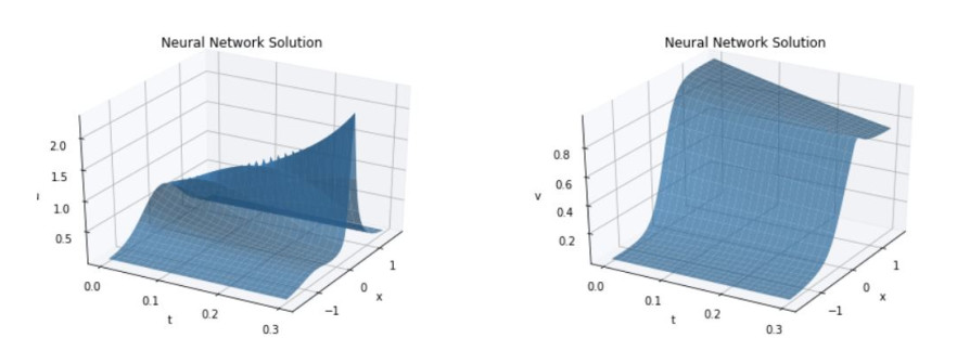
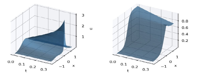
We consider the mathematical model of chemotaxis introduced by Patlak, Keller, and Segel. Aggregation and progression waves are present everywhere in the population dynamics of chemotactic cells. Aggregation originates from the chemotaxis of mobile cells, where cells are attracted to migrate to higher concentrations of the chemical signal region produced by themselves. The neural net can be used to find the approximate solution of the PDE. We proved that the error, the difference between the actual value and the predicted value, is bound to a constant multiple of the loss we are learning. Also, the Neural Net approximation can be easily applied to the inverse problem. It was confirmed that even when the coefficient of the PDE equation was unknown, prediction with high accuracy was achieved.
- differential equation,
- approximated solution,
- artificial neural networks,
- Patlak-Keller-Segel equation
Citation: Sunwoo Hwang, Seongwon Lee, Hyung Ju Hwang. Neural network approach to data-driven estimation of chemotactic sensitivity in the Keller-Segel model[J]. Mathematical Biosciences and Engineering, 2021, 18(6): 8524-8534. doi: 10.3934/mbe.2021421

Related Papers:

Abstract

We consider the mathematical model of chemotaxis introduced by Patlak, Keller, and Segel. Aggregation and progression waves are present everywhere in the population dynamics of chemotactic cells. Aggregation originates from the chemotaxis of mobile cells, where cells are attracted to migrate to higher concentrations of the chemical signal region produced by themselves. The neural net can be used to find the approximate solution of the PDE. We proved that the error, the difference between the actual value and the predicted value, is bound to a constant multiple of the loss we are learning. Also, the Neural Net approximation can be easily applied to the inverse problem. It was confirmed that even when the coefficient of the PDE equation was unknown, prediction with high accuracy was achieved.

References

[1]	P. Devreotes, C. Janetopoulos, Eukaryotic chemotaxis: Distinctions between directional sensing and polarization, J. Biol. Chem., 278 (2003), 20445–20448. doi: 10.1074/jbc.R300010200
[2]	D. V. Zhelev, A. M. Alteraifi, D. Chodniewicz, Controlled pseudopod extension of human neutrophils stimulated with different chemoattractants, Biophys. J., 87 (2004), 688–695. doi: 10.1529/biophysj.103.036699
[3]	E. F. Keller, L. A. Segel, Initiation of slime mold aggregation viewed as an instability, J. Theor. Biol., 26 (1970), 399–415. doi: 10.1016/0022-5193(70)90092-5
[4]	L. A. Segel, A. Goldbeter, P. N. Devreotes, B. E. Knox, A mechanism for exact sensory adaptation based on receptor modification, J. Theor. Biol., 120 (1986), 151–179. doi: 10.1016/S0022-5193(86)80171-0
[5]	J. A. Sherratt, Chemotaxis and chemokinesis in eukaryotic cells: The Keller-Segel equations as an approximation to a detailed model, Bull. Math. Biol., 56 (1994), 129–146. doi: 10.1007/BF02458292
[6]	C. S. Patlak, Random walk with persistence and external bias, Bull. Math. Biophys., 15 (1953), 311–338. doi: 10.1007/BF02476407
[7]	E. F. Keller, L. A. Segel, Model for chemotaxis, J. Theor. Biol., 30 (1971), 225–234. doi: 10.1016/0022-5193(71)90050-6
[8]	E. F. Keller, L. A. Segel, Traveling bands of chemotactic bacteria: a theoretical analysis, J. Theor. Biol., 30 (1971), 235–248. doi: 10.1016/0022-5193(71)90051-8
[9]	H. Jo, H. Son, H. J. Hwang, E. H. Kim, Deep neural network approach to forward-inverse problems, Networks Heterog. Media, 15 (2020), 247. doi: 10.3934/nhm.2020011
[10]	M. Raissi, P. Perdikaris, G. E. Karniadakis, Physics informed deep learning (part i): Data-driven solutions of nonlinear partial differential equations, arXiv: 1711.10561.
[11]	M. Raissi, P. Perdikaris, G. E. Karniadakis, Physics-informed neural networks: A deep learning framework for solving forward and inverse problems involving nonlinear partial differential equations, J. Comput. Phys., 378 (2019), 686–707. doi: 10.1016/j.jcp.2018.10.045
[12]	X. Li, Simultaneous approximations of multivariate functions and their derivatives by neural networks with one hidden layer, Neurocomputing, 12 (1996), 327–343. doi: 10.1016/0925-2312(95)00070-4
[13]	J. Soler, J. A. Carrillo, L. L. Bonilla, Asymptotic behavior of an initial-boundary value problem for the Vlasov–Poisson–Fokker–Planck system, SIAM J. Appl. Math., 57 (1997), 1343–1372. doi: 10.1137/S0036139995291544
[14]	F. Bouchut, J. Dolbeault, On long time asymptotics of the Vlasov-Fokker-Planck equation and of the Vlasov-Poisson-Fokker-Planck system with Coulombic and Newtonian potentials, Differ. Integral Equat., 8 (1995), 487–514.
[15]	J. Han, A. Jentzen, E. Weinan, Solving high-dimensional partial differential equations using deep learning, Proceed. Nat. Aca. Sci., 115 (2018), 8505–8510. doi: 10.1073/pnas.1718942115
[16]	J. Bourgain, Fourier transform restriction phenomena for certain lattice subsets and applications to nonlinear evolution equations, Geometric & Functional Analysis GAFA, 3 (1993), 209–262.
[17]	H. J. Hwang, J. W. Jang, H. Jo, J. Y. Lee, Trend to equilibrium for the kinetic Fokker-Planck equation via the neural network approach, J. Comput. Phys., 419 (2020), 109665. doi: 10.1016/j.jcp.2020.109665
[18]	Clawpack Development Team, Clawpack software, http://www.clawpack.org, Version 5.5.0, (2018).
[19]	K. T. Mandli, A. J. Ahmadia, M. Berger, D. Calhoun, D. L. George, Y. Hadjimichael, et al., Clawpack: Building an open source ecosystem for solving hyperbolic PDEs, PeerJ Comput. Sci., 2 (2016), e68. doi: 10.7717/peerj-cs.68
[20]	R. Tyson, L. G. Stern, R. J. LeVeque, Fractional step methods applied to a chemotaxis model, J. Math. Biol., 41 (2000), 455–475. doi: 10.1007/s002850000038

Reader Comments

Your name:*

Email:*
© 2021 the Author(s), licensee AIMS Press. This is an open access article distributed under the terms of the Creative Commons Attribution License (http://creativecommons.org/licenses/by/4.0)