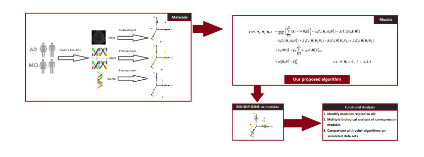
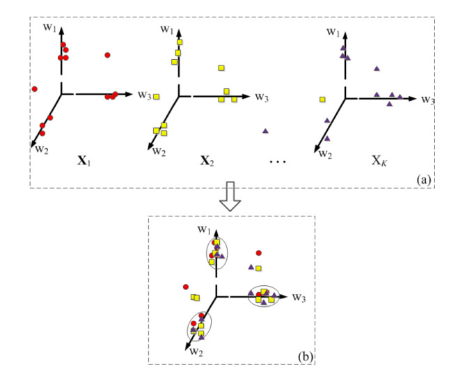
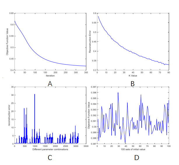
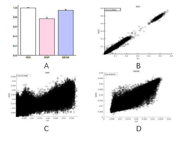
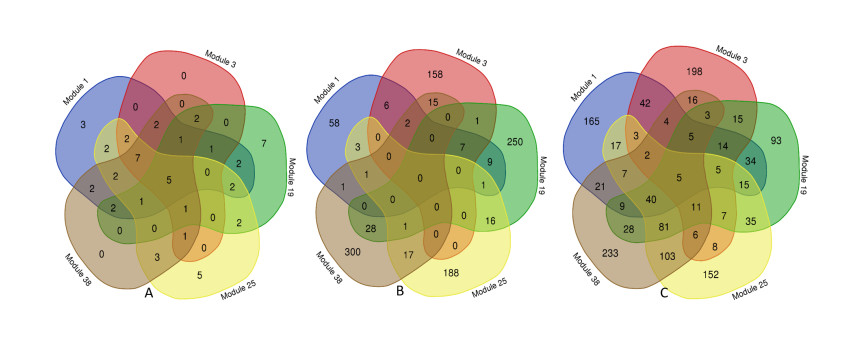
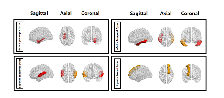
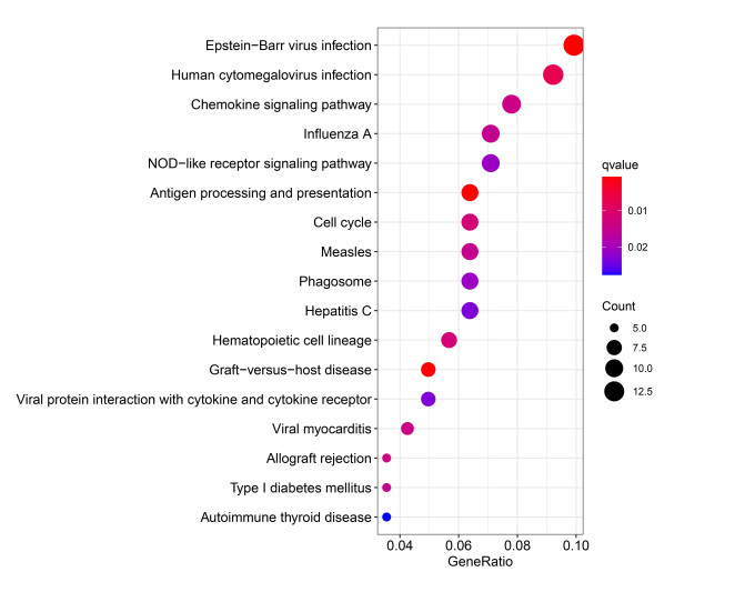
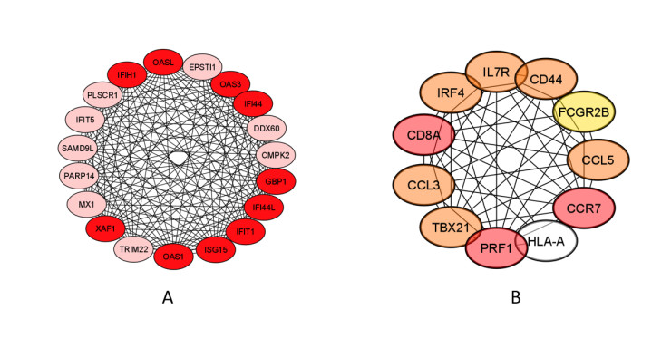
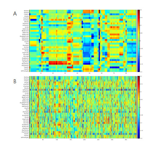
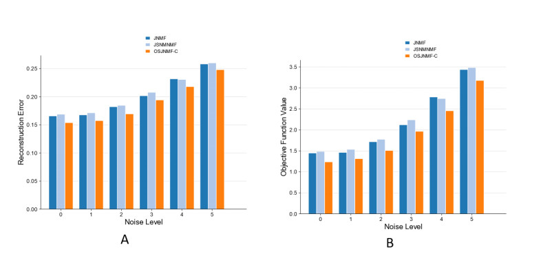
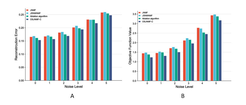
Based on the mining of micro- and macro-relationships of genetic variation and brain imaging data, imaging genetics has been widely applied in the early diagnosis of Alzheimer's disease (AD). However, effective integration of prior knowledge remains a barrier to determining the biological mechanism of AD. This paper proposes a new connectivity-based orthogonal sparse joint non-negative matrix factorization (OSJNMF-C) method based on integrating the structural magnetic resonance image, single nucleotide polymorphism and gene expression data of AD patients; the correlation information, sparseness, orthogonal constraint and brain connectivity information between the brain image data and genetic data are designed as constraints in the proposed algorithm, which efficiently improved the accuracy and convergence through multiple iterative experiments. Compared with the competitive algorithm, OSJNMF-C has significantly smaller related errors and objective function values than the competitive algorithm, showing its good anti-noise performance. From the biological point of view, we have identified some biomarkers and statistically significant relationship pairs of AD/mild cognitive impairment (MCI), such as rs75277622 and BCL7A, which may affect the function and structure of multiple brain regions. These findings will promote the prediction of AD/MCI.
Citation: Wei Kong, Feifan Xu, Shuaiqun Wang, Kai Wei, Gen Wen, Yaling Yu. Application of orthogonal sparse joint non-negative matrix factorization based on connectivity in Alzheimer's disease research[J]. Mathematical Biosciences and Engineering, 2023, 20(6): 9923-9947. doi: 10.3934/mbe.2023435
Based on the mining of micro- and macro-relationships of genetic variation and brain imaging data, imaging genetics has been widely applied in the early diagnosis of Alzheimer's disease (AD). However, effective integration of prior knowledge remains a barrier to determining the biological mechanism of AD. This paper proposes a new connectivity-based orthogonal sparse joint non-negative matrix factorization (OSJNMF-C) method based on integrating the structural magnetic resonance image, single nucleotide polymorphism and gene expression data of AD patients; the correlation information, sparseness, orthogonal constraint and brain connectivity information between the brain image data and genetic data are designed as constraints in the proposed algorithm, which efficiently improved the accuracy and convergence through multiple iterative experiments. Compared with the competitive algorithm, OSJNMF-C has significantly smaller related errors and objective function values than the competitive algorithm, showing its good anti-noise performance. From the biological point of view, we have identified some biomarkers and statistically significant relationship pairs of AD/mild cognitive impairment (MCI), such as rs75277622 and BCL7A, which may affect the function and structure of multiple brain regions. These findings will promote the prediction of AD/MCI.

| [1] | E. Parkhomenko, D. Tritchler, J. Beyene, Sparse canonical correlation analysis with application to genomic data integration, Stat. Appl. Genet. Mol. Biol., 2009 (2009). https://doi.org/10.2202/1544-6115.1406 |
| [2] |
P. Peng, Y. Zhang, Y. Ju, K. Wang, G. Li, V. Calhoun, et al., Group sparse joint non-negative matrix factorization on orthogonal subspace for multi-modal imaging genetics data analysis, IEEE/ACM Trans. Comput. Biol. Bioinf., 19 (2022), 479–490. https://doi.org/10.1109/TCBB.2020.2999397 doi: 10.1109/TCBB.2020.2999397

|
| [3] |
S. Zhang, C. Liu, W. Li, H. Shen, P. Laird, X. Zhou, Discovery of multi-dimensional modules by integrative analysis of cancer genomic data, Nucleic Acids Res., 40 (2012), 9379–9391. https://doi.org/10.1093/nar/gks725 doi: 10.1093/nar/gks725
|
| [4] |
S. Zhang, Q. Li, J. Liu, X. Zhou, A novel computational framework for simultaneous integration of multiple types of genomic data to identify microRNA-gene regulatory modules, Bioinformatics., 27 (2011), 401–409. https://doi.org/10.1093/bioinformatics/btr206 doi: 10.1093/bioinformatics/btr206
|
| [5] |
J. Deng, W. Kong, S. Wang, X. Mou, W. Zeng, Prior knowledge driven joint NMF algorithm for ceRNA co-module identification, Int. J. Biol. Sci., 14 (2018), 1822–1833. https://doi.org/10.7150/ijbs.27555 doi: 10.7150/ijbs.27555
|
| [6] |
M. Wang, T. Huang, J. Fang, V. Calhoun, Y. Wang, Integration of imaging (epi) genomics data for the study of schizophrenia using group sparse joint nonnegative matrix factorization, IEEE/ACM Trans. Comput. Biol. Bioinf., 17 (2020), 1671–1681. https://doi.org/10.1109/TCBB.2019.2899568 doi: 10.1109/TCBB.2019.2899568
|
| [7] |
H. Kim, H. Park, Sparse non-negative matrix factorizations via alternating non-negativity-constrained least squares for microarray data analysis, Bioinformatics, 23 (2007), 1495–1502. https://doi.org/10.1093/bioinformatics/btm134 doi: 10.1093/bioinformatics/btm134
|
| [8] |
J. Deng, W. Zeng, W. Kong, Y. Shi, X. Mou, J. Guo, Multi-constrained joint non-negative matrix factorization with application to imaging genomic study of lung metastasis in soft tissue sarcomas, IEEE Trans. Biomed. Eng., 67 (2020), 2110–2118. https://doi.org/10.1109/TBME.2019.2954989 doi: 10.1109/TBME.2019.2954989
|
| [9] |
J. Deng, W. Zeng, S. Luo, W. Kong, Y. Shi, Y. Li, et al., Integrating multiple genomic imaging data for the study of lung metastasis in sarcomas using multi-dimensional constrained joint non-negative matrix factorization, Inf. Sci., 576 (2021), 24–36. https://doi.org/10.1016/j.ins.2021.06.058 doi: 10.1016/j.ins.2021.06.058
|
| [10] | M. Kim, J. Won, J. Youn, H. Park, Joint-connectivity-based sparse canonical correlation analysis of imaging genetics for detecting biomarkers of Parkinson's disease, IEEE Trans. Med. Imaging, 39 (2020), 23–34. |
| [11] |
K. Wei, W. Kong, S. Wang, Integration of imaging genomics data for the study of Alzheimer's disease using joint-connectivity-based sparse nonnegative matrix factorization, J. Mol. Neurosci., 72 (2022), 255–272. https://doi.org/10.1007/s12031-021-01888-6 doi: 10.1007/s12031-021-01888-6
|
| [12] |
K. Wei, W. Kong, S. Wang, An improved multi-task sparse canonical correlation analysis of imaging genetics for detecting biomarkers of Alzheimer's disease, IEEE Access, 9 (2021), 30528– 30538. https://doi.org/10.1109/ACCESS.2021.3059520 doi: 10.1109/ACCESS.2021.3059520
|
| [13] |
S. Purcell, B. Neale, K. Brown, L. Thomas, M. Ferreira, D. Bender, et al., PLINK: A tool set for whole-genome association and population-based linkage analyses, Am. J. Hum. Genet., 81 (2007), 559–575. https://doi.org/10.1086/519795 doi: 10.1086/519795
|
| [14] | M. Ritchie, B. Phipson, D. Wu, Y. Hu, C. Law, W. Shi, et al., Limma powers differential expression analyses for RNA-sequencing and microarray studies, Nucleic Acids Res., 43 (2015). https://doi.org/10.1093/nar/gkv007 |
| [15] |
J. Liu, X. Zhang, C. Yu, Y. Duan, J. Zhuo, Y. Cui, et al., Impaired parahippocampus connectivity in mild cognitive impairment and Alzheimer's disease, J. Alzheimers Dis., 49 (2016), 1051–1064. https://doi.org/10.3233/JAD-150727 doi: 10.3233/JAD-150727
|
| [16] |
J. Sun, J. Maller, L. Guo, P. Fitzgerald, Superior temporal gyrus volume change in schizophrenia: a review on region of interest volumetric studies, Brain Res. Rev., 61 (2009), 14–32. https://doi.org/10.1016/j.brainresrev.2009.03.004 doi: 10.1016/j.brainresrev.2009.03.004
|
| [17] |
S. Scheff, D. Price, F. Schmitt, M. Scheff, E. Mufson, Synaptic loss in the inferior temporal gyrus in mild cognitive impairment and Alzheimer's disease, J. Alzheimers Dis., 24 (2011), 547–557. https://doi.org/10.3233/JAD-2011-101782 doi: 10.3233/JAD-2011-101782
|
| [18] |
N. Bezuch, S. Bradburn, A. Robinson, N. Pendleton, A. Payton, C. Murgatroyd, Superior frontal gyrus TOMM40-APOELocus DNA methylation in Alzheimer's disease, J. Alzheimers Dis. Rep., 5 (2021), 275–282. https://doi.org/10.3233/ADR-201000 doi: 10.3233/ADR-201000
|
| [19] | M. Xia, J. Wang, Y. He, BrainNet viewer: A network visualization tool for human brain connectomics, Plos One, 8 (2013). https://doi.org/10.1371/journal.pone.0068910 |
| [20] | C. M. Karch, L. A. Ezerskiy, S. Bertelsen, A. M. Goate, Alzheimer's disease risk polymorphisms regulate gene expression in the ZCWPW1 and the CELF1 loci, Plos One, 11 (2016). https://doi.org/10.1371/journal.pone.0148717 |
| [21] |
J. H. Kim, Genetics of Alzheimer's Disease, Dementia Neurocogn. Disord., 17 (2018), 131–136. https://doi.org/10.12779/dnd.2018.17.4.131 doi: 10.12779/dnd.2018.17.4.131
|
| [22] |
E. van der Ende, L. Meeter, C. Stingl, J. van Rooij, M. P. Stoop, D. Nijholt, et al., Novel CSF biomarkers in genetic frontotemporal dementia identified by proteomics, Ann. Clin. Transl. Neurol., 6 (2019), 698–707. https://doi.org/10.1002/acn3.745 doi: 10.1002/acn3.745
|
| [23] |
S. Ochi, J. Iga, Y. Funahashi, Y. Yoshino, K. Yamazaki, H. Kumon, et al., Identifying blood transcriptome biomarkers of Alzheimer's disease using transgenic mice, Mol. Neurobiol., 57 (2020), 4941–4951. https://doi.org/10.1007/s12035-020-02058-2 doi: 10.1007/s12035-020-02058-2
|
| [24] | C. Lin, E. Lin, H. Lane, Genetic biomarkers on age-related cognitive decline, Front. Psychiatry, 8 (2017). https://doi.org/10.3389/fpsyt.2017.00247 |
| [25] | R. Armstrong, Risk factors for Alzheimer's disease, Folia Neuropathol., 57 (2019), 87–105. |
| [26] |
M. J. Chen, S. Ramesha, L. D. Weinstock, T. W. Gao, L. Y. Ping, H. L. Xiao, et al., Extracellular signal-regulated kinase regulates microglial immune responses in Alzheimer's disease, J. Neurosci. Res., 99 (2021), 1704–1721. https://doi.org/10.1002/jnr.24829 doi: 10.1002/jnr.24829
|
| [27] |
A. de Roeck, C. van Broeckhoven, K. Sleegers, The role of ABCA7 in Alzheimer's disease: evidence from genomics, transcriptomics and methylomics, Acta Neuropathol., 138 (2019), 201–220. https://doi.org/10.1007/s00401-019-01994-1 doi: 10.1007/s00401-019-01994-1
|
| [28] |
N. Kim, L. Yu, R. Dawe, V. A. Petyuk, C. Gaiteri, P. L. Jager, et al., Microstructural changes in the brain mediate the association of AK4, IGFBP5, HSPB2, and ITPK1 with cognitive decline, Neurobiol. Aging, 84 (2019), 17–25. https://doi.org/10.1016/j.neurobiolaging.2019.07.013 doi: 10.1016/j.neurobiolaging.2019.07.013
|
| [29] | R. Shen, X. Zhao, L. He, Y. Ding, W. Xu, S. Lin, et al., Upregulation of RIN3 induces endosomal dysfunction in Alzheimer's disease, Transl. Neurodegener., 9 (2020). https://doi.org/10.1186/s40035-020-00206-1 |
| [30] |
A. S. Pozo, S. Das, B. T. Hyman, APOE and Alzheimer's disease: advances in genetics, pathophysiology, and therapeutic approaches, Lancet Neurol., 20 (2021), 68–80. https://doi.org/10.1016/S1474-4422(20)30412-9 doi: 10.1016/S1474-4422(20)30412-9
|
| [31] |
M. E. Belloy, V. Napolioni, M. D. Greicius, A quarter century of APOE and Alzheimer's disease: Progress to date and the path forward, Neuron, 101 (2019), 820–838. https://doi.org/10.1016/j.neuron.2019.01.056 doi: 10.1016/j.neuron.2019.01.056
|
| [32] |
J. Bratosiewicz-Wasik, P. P. Liberski, B. Peplonska, M. Styczynska, J. Smolen-Dzirba, M. Cycon, et al., Regulatory region single nucleotide polymorphisms of the apolipoprotein E gene as risk factors for Alzheimer's disease, Neurosci. Lett., 684 (2018), 86–90. https://doi.org/10.1016/j.neulet.2018.07.010 doi: 10.1016/j.neulet.2018.07.010
|
| [33] | A. A. Assareh, O. Piguet, T. C. Lye, K. A. Mather, G. A. Broe, P. R. Schofield, et al., Association of SORL1 gene variants with hippocampal and cerebral atrophy and Alzheimerµs disease, Curr. Alzheimer Res., 11 (2014), 558–563. |
| [34] | S. Seshadri, A. L. DeStefano, R. Au, J. M. Massaro, A. S. Beiser, M. Kelly-Hayes, et al., Genetic correlates of brain aging on MRI and cognitive test measures: a genome-wide association and linkage analysis in the Framingham study, BMC Med. Genet., 8 (2007). https://doi.org/10.1186/1471-2350-8-S1-S15 |
| [35] |
S. A. Krynskiy, I. K. Malashenkova, D. P. Ogurtsov, N. A. Khailov, E. I. Chekulaeva, O. Y. Shipulina, et al., Herpesvirus infections and immunological disturbances in patients with different stages of Alzheimer's disease, Probl. Virol., 66 (2021), 129–139. https://doi.org/10.36233/0507-4088-32 doi: 10.36233/0507-4088-32
|
| [36] |
D. L. Ewins, M. N. Rossor, J. Butler, P. K. Roques, M. J. Mullan, A. M. McGregor, Association between autoimmune thyroid disease and familial Alzheimer's disease, Clin. Endocrinol., 35 (1991), 93–96. https://doi.org/10.1111/j.1365-2265.1991.tb03502.x doi: 10.1111/j.1365-2265.1991.tb03502.x
|
| [37] | P. Suresh, S. Phasuk, I. Y. Liu, Modulation of microglia activation and Alzheimer's disease: CX3 chemokine ligand 1/CX3CR and P2X7R signaling, Tzu Chi Med. J., 33 (2021), 1–6. |
| [38] |
B. Popp, A. B. Ekici, C. T. Thiel, J. Hoyer, A. Wiesener, C. Kraus, et al., Exome Pool-Seq in neurodevelopmental disorders, Eur. J. Hum. Genet., 25 (2017), 1364–1376. https://doi.org/10.1038/s41431-017-0022-1 doi: 10.1038/s41431-017-0022-1
|
| [39] |
S. Desai, M. Juncker, C. Kim, Regulation of mitophagy by the ubiquitin pathway in neurodegenerative diseases, Exp. Biol. Med., 243 (2018), 554–562. https://doi.org/10.1177/1535370217752351 doi: 10.1177/1535370217752351
|
| [40] | D. A. Salih, S. Bayram, S. Guelfi, R. H. Reynolds, M. Shoai, M. Ryten, et al., Genetic variability in response to amyloid beta deposition influences Alzheimer's disease risk, Brain Commun., 1 (2019). https://doi.org/10.1093/braincomms/fcz022 |
| [41] | R. A. Cifuentes, J. Murillo-Rojas, Alzheimer's disease and HLA-A2: linking neurodegenerative to immune processes through an in silico approach, Biomed Res. Int., 2014 (2014). https://doi.org/10.1155/2014/791238 |
| [42] | S. da Mesquita, J. Herz, M. Wall, T. Dykstra, K. A. Lima, G. T. Norris, et al., Aging-associated deficit in CCR7 is linked to worsened glymphatic function, cognition, neuroinflammation, and $\beta$-amyloid pathology, Sci. Adv., 7 (2021). https://doi.org/10.1126/sciadv.abe4601 |
| [43] |
M. G. Kitzbichler, A. R. Aruldass, G. J. Barker, T. C. Wood, N. G. Dowell, S. A. Hurley, et al., Peripheral inflammation is associated with micro-structural and functional connectivity changes in depression-related brain networks, Mol. Psychiatry, 26 (2021), 7346–7354. https://doi.org/10.1038/s41380-021-01272-1 doi: 10.1038/s41380-021-01272-1
|
| [44] |
X. Wang, X. Cui, C. Ding, D. Li, C. Cheng, B. Wang, et al., Deficit of cross‐frequency integration in mild cognitive impairment and Alzheimer's disease: A multilayer network approach, J. Magn. Reson. Imaging, 53 (2021), 1387–1398. https://doi.org/10.1002/jmri.27453 doi: 10.1002/jmri.27453
|
| [45] | Y. Mao, Z. Liao, X. Liu, T. Li, J. Hu, D. Le, et al., Disrupted balance of long and short-range functional connectivity density in Alzheimer's disease (AD) and mild cognitive impairment (MCI) patients: a resting-state fMRI study, Ann. Transl. Med., 9 (2021). https://doi.org/10.21037/atm-20-7019 |
| [46] |
Y. Chang, J. Hsu, S. Huang, S. Hsu, C. Lee, C. Chang, Functional connectome and neuropsychiatric symptom clusters of Alzheimer's disease, J. Affect Disord., 273 (2020), 48–54. https://doi.org/10.1016/j.jad.2020.04.054 doi: 10.1016/j.jad.2020.04.054
|
| [47] |
R. J. Vanzo, H. Twede, K. S. Ho, A. Prasad, M. M. Martin, S. T. South, et al., Clinical significance of copy number variants involving KANK1 in patients with neurodevelopmental disorders, Eur. J. Med. Genet., 62 (2019), 15–20. https://doi.org/10.1016/j.ejmg.2018.04.012 doi: 10.1016/j.ejmg.2018.04.012
|
| [48] | S. Soleimani, N. Nasim, F. Esfandi, M. Karimipoor, V. K. Oskooei, M. N. Gol, et al., SE translocation gene but not zinc finger or X-linked factor is down-regulated in gastric cancer, Gastroenterol. Hepatol. Bed Bench, 13 (2020), 8–13. |
Figures(11) / Tables(4)

Wei Kong, Feifan Xu, Shuaiqun Wang, Kai Wei, Gen Wen, Yaling Yu. Application of orthogonal sparse joint non-negative matrix factorization based on connectivity in Alzheimer's disease research[J]. Mathematical Biosciences and Engineering, 2023, 20(6): 9923-9947. doi: 10.3934/mbe.2023435


 DownLoad: