Linear barycentric rational collocation method for solving generalized Poisson equations

Jin Li; Yongling Cheng; Zongcheng Li; Zhikang Tian; Jin Li; Yongling Cheng; Zongcheng Li; Zhikang Tian

doi:10.3934/mbe.2023221

Mathematical Biosciences and Engineering

2023, Volume 20, Issue 3: 4782-4797. doi: 10.3934/mbe.2023221

Previous Article Next Article

Research article Special Issues

Linear barycentric rational collocation method for solving generalized Poisson equations

1.
School of Science, Shandong Jianzhu University, No. 1000 Fengming Road, Lingang Development Zone, Jinan 250101, Shandong, China
2.
Lab Master at School of Computer Science and Technology, Shandong Jianzhu University, No. 1000 Fengming Road, Lingang Development Zone, Jinan 250101, Shandong, China

Academic Editor: Feliz Minhós

Received: 29 November 2022 Revised: 19 December 2022 Accepted: 21 December 2022 Published: 03 January 2023

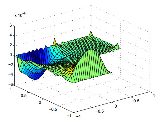
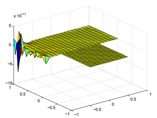
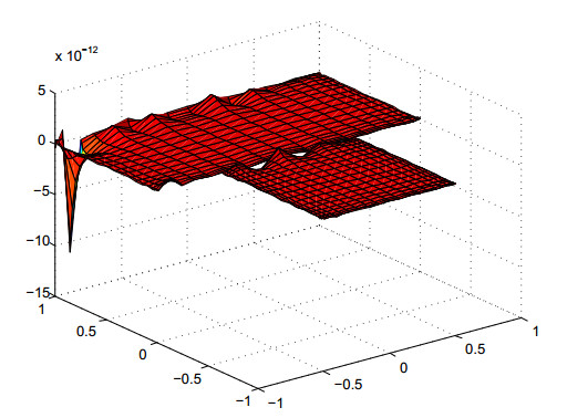
We consider the Poisson equation by collocation method with linear barycentric rational function. The discrete form of the Poisson equation was changed to matrix form. For the basis of barycentric rational function, we present the convergence rate of the linear barycentric rational collocation method for the Poisson equation. Domain decomposition method of the barycentric rational collocation method (BRCM) is also presented. Several numerical examples are provided to validate the algorithm.

Keywords:

Citation: Jin Li, Yongling Cheng, Zongcheng Li, Zhikang Tian. Linear barycentric rational collocation method for solving generalized Poisson equations[J]. Mathematical Biosciences and Engineering, 2023, 20(3): 4782-4797. doi: 10.3934/mbe.2023221

Related Papers:

[1]	Jin Li . Linear barycentric rational collocation method to solve plane elasticity problems. Mathematical Biosciences and Engineering, 2023, 20(5): 8337-8357. doi: 10.3934/mbe.2023365
[2]	Wenting Li, Ailing Jiao, Wei Liu, Zhaoying Guo . High-order rational-type solutions of the analogous (3+1)-dimensional Hirota-bilinear-like equation. Mathematical Biosciences and Engineering, 2023, 20(11): 19360-19371. doi: 10.3934/mbe.2023856
[3]	Ishtiaq Ali . Bernstein collocation method for neutral type functional differential equation. Mathematical Biosciences and Engineering, 2021, 18(3): 2764-2774. doi: 10.3934/mbe.2021140
[4]	Andras Balogh, Tamer Oraby . Stochastic games of parental vaccination decision making and bounded rationality. Mathematical Biosciences and Engineering, 2025, 22(2): 355-388. doi: 10.3934/mbe.2025014
[5]	Baojian Hong . Bifurcation analysis and exact solutions for a class of generalized time-space fractional nonlinear Schrödinger equations. Mathematical Biosciences and Engineering, 2023, 20(8): 14377-14394. doi: 10.3934/mbe.2023643
[6]	Bruno Buonomo, Alberto d’Onofrio, Deborah Lacitignola . Rational exemption to vaccination for non-fatal SIS diseases: Globally stable and oscillatory endemicity. Mathematical Biosciences and Engineering, 2010, 7(3): 561-578. doi: 10.3934/mbe.2010.7.561
[7]	Alessia Andò, Simone De Reggi, Davide Liessi, Francesca Scarabel . A pseudospectral method for investigating the stability of linear population models with two physiological structures. Mathematical Biosciences and Engineering, 2023, 20(3): 4493-4515. doi: 10.3934/mbe.2023208
[8]	Max-Olivier Hongler, Roger Filliger, Olivier Gallay . Local versus nonlocal barycentric interactions in 1D agent dynamics. Mathematical Biosciences and Engineering, 2014, 11(2): 303-315. doi: 10.3934/mbe.2014.11.303
[9]	Mario Lefebvre . An optimal control problem without control costs. Mathematical Biosciences and Engineering, 2023, 20(3): 5159-5168. doi: 10.3934/mbe.2023239
[10]	Dimitri Breda, Davide Liessi . A practical approach to computing Lyapunov exponents of renewal and delay equations. Mathematical Biosciences and Engineering, 2024, 21(1): 1249-1269. doi: 10.3934/mbe.2024053

Abstract

1. Introduction

Two-dimensional elliptic ^[1] boundary value problems

$\begin{eqnarray} \frac{\partial}{\partial t}\left(a(t,s)\frac{\partial u(t, s)}{\partial t}\right)+ \frac{\partial}{\partial s}\left(b(t,s)\frac{\partial u(t, s)}{\partial s}\right) = f(t,s),(t,s) \in \Omega \end{eqnarray}$

(1.1)

with

$\begin{eqnarray} u(t,s) = g(t,s), \quad \frac{\partial u(t, s)}{\partial n} = h(t,s), \quad(t,s) \in \partial \Omega, \end{eqnarray}$

(1.2)

where $\Omega = [a, b] \times[c, d]$ and $f(t, s), g(t, s), h(t, s)$ on $\Omega$ , can be used in many scientific areas, such as electrostatics, mechanical engineering, magnetic fields, thermal fields and brain activity detection^[2].

Floater ^[3,4,5] proposed a rational interpolation scheme. In ^[6], a linear rational collocation method was presented for the lower regular function. Wang et al.^[7,8,9,10] successfully solved initial value problems, plane elasticity problems, incompressible plane problems and non-linear problems by collocation method. The linear barycentric rational collocation method (LBRCM) to solve nonlinear parabolic partial differential equations^[11], biharmonic equation ^[12], fractional differential equations^[13], telegraph equation ^[14], Volterra integro-differential equation ^[15] and heat conduction equation^[16] have been studied.

In the following, we introduce the barycentric formula of a one dimensional function. Let

$\begin{eqnarray} p(t) = \sum\limits_{j = 1}^{n} L_{j}(t) f_{j}, \end{eqnarray}$

(1.3)

and

$\begin{eqnarray} L_{j}(t) = \frac{ \prod\limits_{k = 1, k \neq j}^{n}\left(t-t_{k}\right)}{ \prod\limits_{k = 1, k \neq j}^{n}\left(t_{j}-t_{k}\right)}. \end{eqnarray}$

(1.4)

In order to get the barycentric formula, Eq (1.4) is changed into

$\begin{eqnarray} l(t) = \left(t-t_{1}\right)\left(t-t_{2}\right) \cdots\left(t-t_{n}\right) \end{eqnarray}$

(1.5)

and

$\begin{eqnarray} w_{j} = \frac{1}{\prod_{j \neq k}\left(t_{j}-t_{k}\right)}, \quad j = 1,2, \cdots, n, \end{eqnarray}$

(1.6)

which means $w_{j} = 1 / l^{\prime}(t_{j})$ .

$\begin{eqnarray} L_{j}(t) = l(t) \frac{w_{j}}{t-t_{j}}, \quad j = 1,2, \cdots, n. \end{eqnarray}$

(1.7)

For Eq (1.2), we get

$\begin{eqnarray} p(t) = l(t) \sum\limits_{j = 1}^{n} \frac{w_{j}}{t-t_{j}} f_{j} \end{eqnarray}$

(1.8)

which means

$\begin{eqnarray} p(t) = \frac{ \sum\limits_{j = 1}^{n}\frac{w_{j}}{t-t_{j}} f_{j}}{ \sum\limits_{j = 1}^{n} \frac{w_{j}}{t-t_{j}}}. \end{eqnarray}$

(1.9)

For the case uniform partition, we get

$\begin{eqnarray} w_{j} = (-1)^{n-j} C_{n}^{j} = (-1)^{n-j} \frac{n!}{j!(n-j)!}. \end{eqnarray}$

(1.10)

For the case the nonuniform partition is chosen, we take the second Chebyshev point ^[7] a

$\begin{eqnarray} t_{j} = \cos \frac{(j-1) \pi}{n-1}, \quad j = 1, \cdots, n \end{eqnarray}$

(1.11)

with

$\begin{eqnarray} w_{j} = (-1)^{j} \delta_{j}, \quad \delta_{j} = \left\{\begin{array}{l}{1 / 2},j = 1,n \\ {1}, otherwise \end{array}\right. \end{eqnarray}$

(1.12)

For the barycentric rational function, we first set

$\begin{eqnarray} r(t) = \frac{ \sum\limits_{i = 1}^{n-d} \lambda_{i}(t) p_{i}(t)} { \sum\limits_{i = 1}^{n-d} \lambda_{i}(t)} \end{eqnarray}$

(1.13)

where

$\begin{eqnarray} \lambda_{i}(t) = \frac{(-1)^{i}}{\left(t-t_{i}\right) \cdots\left(t-t_{i+d}\right)} \end{eqnarray}$

(1.14)

and

$\begin{eqnarray} p_{i}(t) = \sum\limits_{k = i}^{i+d} \prod\limits_{j = i, j \neq k}^{i+d} \frac{t-t_{j}}{t_{k}-t_{j}} f_{k}. \end{eqnarray}$

(1.15)

Combining (1.14) and (1.15), we have

$\begin{eqnarray} \sum\limits_{i = 1}^{n-d} \lambda_{i}(t) p_{i}(t) = \sum\limits_{i = 1}^{n-d}(-1)^{i} \sum\limits_{k = i}^{i+d} \frac{1}{t-t_{k}} \prod\limits_{i, j \neq k}^{i+d} \frac{1}{t_{k}-t_{j}} f_{k} = \sum\limits_{k = 1}^{n} \frac{w_{k}}{t-t_{k}} f_{k} \end{eqnarray}$

(1.16)

where

$\begin{eqnarray} w_{k} = \sum\limits_{i \in J_{k}}(-1)^{i} \prod\limits_{j = i, j \neq k}^{i+d} \frac{1}{t_{k}-t_{j}} \end{eqnarray}$

(1.17)

and $J_{k} = \{i \in I; k-d \leqslant i \leqslant k\}$ . By taking $p(t) = 1$ , we have

$\begin{eqnarray} 1 = \sum\limits_{k = i}^{i+d} \prod\limits_{j = i, j \neq k}^{i+d} \frac{t-t_{j}}{t_{k}-t_{j}} \end{eqnarray}$

(1.18)

and then have

$\begin{eqnarray} \sum\limits_{i = 1}^{n-d} \lambda_{i}(t) = \sum\limits_{k = 1}^{n} \frac{w_{k}}{t-t_{k}}. \end{eqnarray}$

(1.19)

Combining (1.16), (1.19) and (1.13), we get

$\begin{eqnarray} r(t) = \frac{ \sum\limits_{j = 1}^{n} \frac{w_{j}}{t-t_{j}} f_{j}}{ \sum\limits_{j = 1}^{n} \frac{w_{j}}{t-t_{j}}} \end{eqnarray}$

(1.20)

where $\omega_{j}$ is defined as in (1.17).

In this paper, based on linear barycentric rational interpolation of one dimension, we construct a barycentric rational interpolation of a two-dimensional Poisson equation. In order to get the discrete linear equation of a two-dimensional Poisson equation, the equidistant nodes and second kind of Chebyshev points were chosen as collocation point. For the general area, a domain decomposition method of the barycentric rational collocation method is also presented.

2. Differentiation matrices of Poisson equation

Let $a = t_{1} < \cdots < t_{m} = b, h = \frac{b-a}{m}$ and $c = s_{1} < \cdots < s_{n} = d, \tau = \frac{d-c}{n}$ with mesh point $(t_{i}, s_{j}), i = 1, 2, \cdots, m; j = 1, 2, \cdots, n$ . Then, we have

$\begin{eqnarray} u\left(t_{i}, s\right) = u_{i}(s), \end{eqnarray}$

(2.1)

on $[a, b]$ , and

$\begin{eqnarray} u(t,s) = \sum\limits_{i = 1}^{m}\sum\limits_{j = 1}^{n} L_{i}(t) M_{j}(s) u_{ij} \end{eqnarray}$

(2.2)

where

$\begin{eqnarray} L_{i}(t) = \frac{ \frac{w_{i}}{t-t_{i}} }{ \sum\limits_{j = 1}^{n} \frac{w_{j}}{t-t_{j}}} \end{eqnarray}$

(2.3)

and

$\begin{eqnarray} M_{j}(s) = \frac{ \frac{v_{j}}{s-s_{j}} }{ \sum\limits_{j = 1}^{n} \frac{v_{j}}{s-s_{j}}}. \end{eqnarray}$

(2.4)

$w_{i}, v_{j}$ is the weight function defined as (1.6) or (1.17); see ^[17].

We have

$\left[\begin{array}{c}{\sum_{k = 1}^{n} M_{k}^{\prime \prime}\left(s\right) u_{1 k}} \\ {\vdots} \\ {\sum_{k = 1}^{n} M_{k}^{\prime \prime}\left(s\right) u_{m k}}\end{array}\right]+\left[\begin{array}{ccc}{C_{11}^{(2)}} & {\cdots} & {C_{1 m}^{(2)}} \\ {\vdots} & {} & {\vdots} \\ {C_{m 1}^{(2)}} & {\cdots} & {C_{m n}^{(2)}}\end{array}\right]\left[\begin{array}{c}{\sum_{k = 1}^{n} M_{k}\left(s\right) u_{1 k}} \\ {\vdots} \\ {\sum_{k = 1}^{n} M_{k}\left(s\right) u_{m k}}\end{array}\right] = \left[\begin{array}{c}{f_{1}\left(s\right)} \\ {\vdots} \\ {f_{m}\left(s\right)}\end{array}\right].$

Then, we have

$\left[\begin{array}{c}{\sum_{k = 1}^{n} M_{k}^{\prime \prime}\left(s_{j}\right) u_{1 k}} \\ {\vdots} \\ {\sum_{k = 1}^{n} M_{k}^{\prime \prime}\left(s_{j}\right) u_{m k}}\end{array}\right]+\left[\begin{array}{ccc}{C_{11}^{(2)}} & {\cdots} & {C_{1 m}^{(2)}} \\ {\vdots} & {} & {\vdots} \\ {C_{m 1}^{(2)}} & {\cdots} & {C_{m n}^{(2)}}\end{array}\right]\left[\begin{array}{c}{\sum_{k = 1}^{n} M_{k}\left(s_{j}\right) u_{1 k}} \\ {\vdots} \\ {\sum_{k = 1}^{n} M_{k}\left(s_{j}\right) u_{m k}}\end{array}\right] = \left[\begin{array}{c}{f_{1}\left(s_{j}\right)} \\ {\vdots} \\ {f_{m}\left(s_{j}\right)}\end{array}\right],$

where $C_{ij}^{(2)} = L''_{i}(t_{j})$ , and

$\begin{equation} \quad C_{ij}^{(2)} = \left\{\begin{array}{ll}{ 2 L'_{i}(t_{j})\left(L'_{i}(t_{i})-\frac{1}{t_{i}-t_{j}}\right),} & {j \neq i} \\[0.5cm] { -\sum\limits_{i \neq j} L''_{i}(t_{j}),} & {j = i.}\end{array}\right. \end{equation}$

(2.5)

${u}_{i} = \left[u_{i 1}, u_{i 2}, \cdots u_{i n}\right]^{\mathrm{T}}, {f}_{i} = \left[f_{i 1}, f_{i 2}, \cdots, f_{i n}\right]^{\mathrm{T}} = \left[f_{i}\left(s_{i}\right), f_{i}\left(s_{2}\right), \cdots, f_{i}\left(s_{n}\right)\right]^{\mathrm{T}}.$ With the help of the matrix form, the linear equation systems can be written as

$\begin{eqnarray} \left({I}_{m} \otimes {D}^{(2)}\right)\left[\begin{array}{cc}{{u}_{1}} \\ {\vdots} \\ {{u}_{m}}\end{array}\right]+\left({C}^{(2)} \otimes {I}_{n}\right)\left[\begin{array}{c}{{u}_{1}} \\ {\vdots} \\ {{u}_{m}}\end{array}\right] = \left[\begin{array}{c}{f_{1}} \\ {\vdots} \\ {f_{m}}\end{array}\right] \end{eqnarray}$

(2.6)

and $D_{ij}^{(2)} = M''_{i}(s_{j})$ ,

$\begin{equation} \quad D_{ij}^{(2)} = \left\{\begin{array}{ll}{ 2 M'_{i}(s_{j})\left(M'_{i}(s_{i})-\frac{1}{s_{i}-s_{j}}\right),} & {j \neq i,} \\[0.5cm] { -\sum\limits_{i \neq j} M''_{i}(s_{j}),} & {j = i.}\end{array}\right. \end{equation}$

(2.7)

Then, we have

$\begin{eqnarray} \left[\left({C}^{(2)} \otimes {I}_{n}\right)+\left({I}_{m} \otimes {D}^{(2)}\right)\right. ] U = F \end{eqnarray}$

(2.8)

and

$\begin{eqnarray} {L} {U} = {F} \end{eqnarray}$

(2.9)

where

$\begin{eqnarray} L = {C}^{(2)} \otimes {I}_{n}+{I}_{m} \otimes {D}^{(2)} \end{eqnarray}$

(2.10)

and $\otimes$ is the Kronecker product of the matrices. The Kronecker product of $A = (a_{ij})_{m\times n}$ and $B = (b_{ij})_{k\times l}$ is defined as

$\begin{eqnarray} A \times B = (a_{ij}B)_{m\cdot k \times n \cdot l} \end{eqnarray}$

(2.11)

where

$\begin{eqnarray} a_{ij}B = \left[\begin{array}{cccc}{a_{ij} b_{11}} & {a_{ij} b_{12}} & {\cdots} & {a_{ij} b_{1l}} \\ {a_{ij} b_{21}} & {a_{ij} b_{22}} & {\cdots} & {a_{ij} b_{2l}} \\{\vdots} &{\vdots} & {} & {\vdots} \\ {a_{ij} b_{k1}} & {a_{ij} b_{k2}} & {\cdots} & {a_{ij} b_{kl}} \end{array}\right] \end{eqnarray}$

(2.12)

and the node of tensor is $(t_{i}, s_{j}), i = 1, 2, \cdots, \; m; j = 1, 2, \cdots, \; n.$ Then, matrix A and B can be can be changed to $(m\times n)$ column vectors as

$t = [t_{1},\cdots,t_{1},t_{2},\cdots,t_{2},\cdots,t_{m},\cdots,t_{m}]$

$s = [s_{1},s_{2},\cdots,s_{n},s_{1},s_{2},\cdots,s_{n},\cdots,s_{1},s_{2},\cdots,s_{n}],$

and then we get relationship of the partial differential equation and differential matrix as

$\begin{eqnarray} \frac{\partial ^{k+l}u }{\partial ^{k}t\partial ^{l}s} = {C}^{(k)} \otimes {D}^{(l)}, \forall k,l \in N. \end{eqnarray}$

(2.13)

3. Domain decomposition method of barycentric rational collocation method for Poisson equation

Consider the generalized elliptic boundary value problems as

$\begin{eqnarray} \nabla [\beta(t,s) \nabla u(t,s)] = f(t,s),(t,s) \in \Omega \end{eqnarray}$

(3.1)

with boundary condition

$\begin{eqnarray} u(t,s) = u_{0}(t,s),(t,s) \in \Gamma \end{eqnarray}$

(3.2)

where $\beta(t, s)$ is the diffusion coefficient, and $\nabla = \left(\frac{\partial}{ \partial t}, \frac{\partial}{ \partial s}\right)$ is the gradient operator.

Taking the rectangle domain $\Omega$ into two sub-rectangle domains $\Omega_{i}, i = 1, 2$ , the boundary of the domain is $\Gamma$ , and the boundary of $\Omega_{i}, i = 1, 2$ , is $\Gamma_{0}$ . Suppose $\beta(t, s)\in C \Omega$ and the interface conditions of $\Gamma_{0}$ are

$[u]_{\Gamma} = 0,\quad [(\beta\nabla u)\bullet \mathbf{n}]_{\Gamma} = 0.$

Suppose $\beta(t, s)$ is not continuous on $\Omega$ and the interface conditions of $\Gamma_{0}$ are

$[u]_{\Gamma} = \delta(t,s),\quad [(\beta\nabla u)\bullet \mathbf{n}]_{\Gamma} = \gamma(t,s).$

In the following, we take the two sub-domain $\Omega_{i}, i = 1, 2$ , $(t_{1, i}, s_{1, j})$ , the function $u_{1, ij} = u(t_{1, i}, s_{1, j})$ ; $(t_{2, i}, s_{2, j}), i = 1, 2, \cdots, m_{2};j = 1, 2, \cdots, n_{2}$ and $u_{2, ij} = u(t_{2, i}, s_{2, j})$ .

On the sub-domain of $\Omega_{1}$ , the barycentrix function is defined as

$\begin{eqnarray} u(t,s) = \sum\limits_{i = 1}^{m_{1}}\sum\limits_{j = 1}^{n_{1}}R_{1,i}(t)R_{1,j}(s)u_{1,ij} \end{eqnarray}$

(3.3)

where $R_{1, i}(t), R_{1, j}(s)$ are defined as (2.3) and (2.4).

Equation (3.1) can be written as

$\begin{eqnarray} \beta\left(\frac{\partial^2 u}{\partial t^2}+\frac{\partial^2 u}{\partial s^2}\right) +\frac{\partial \beta}{\partial t}\frac{\partial u}{\partial t}+\frac{\partial \beta}{\partial s}\frac{\partial u}{\partial s} = f(t,s),(t,s) \in \Omega \end{eqnarray}$

(3.4)

Taking Eq (3.3) into Eq (3.4), we have

$\begin{eqnarray} &&\beta(t,s)\left(\sum\limits_{i = 1}^{m_{1}}\sum\limits_{j = 1}^{n_{1}}R''_{1,i}(t)R_{1,j}(s)u_{1,ij}+\sum\limits_{i = 1}^{m_{1}}\sum\limits_{j = 1}^{n_{1}}R_{1,i}(t)R''_{1,j}(s)u_{1,ij} \right) \\&&+\frac{\partial \beta(t,s)}{\partial t}\sum\limits_{i = 1}^{m_{1}}\sum\limits_{j = 1}^{n_{1}}R'_{1,i}(t)R_{1,j}(s)u_{1,ij} \\&&+ \frac{\partial \beta(t,s)}{\partial s}\sum\limits_{i = 1}^{m_{1}}\sum\limits_{j = 1}^{n_{1}}R_{1,i}(t)R'_{1,j}(s)u_{1,ij} = f(t,s),(t,s) \in \Omega \end{eqnarray}$

(3.5)

Taking $(t_{1, i}, s_{1, j})$ on the sub-domain of $\Omega_{1}$ , we have

$\begin{eqnarray} &&\beta(t_{1,k},s_{1,l})\left(\sum\limits_{i = 1}^{m_{1}}\sum\limits_{j = 1}^{n_{1}}R''_{1,i}(t_{1,k})R_{1,j}(s_{1,l})u_{1,ij} +\sum\limits_{i = 1}^{m_{1}}\sum\limits_{j = 1}^{n_{1}}R_{1,i}(t_{1,k})R''_{1,j}(s_{1,l})u_{1,ij} \right) \\&&+\frac{\partial \beta(t_{1,k},s_{1,l})}{\partial t}\sum\limits_{i = 1}^{m_{1}}\sum\limits_{j = 1}^{n_{1}}R'_{1,i}(t_{1,k})R_{1,j}(s_{1,l})u_{1,ij} \\&&+ \frac{\partial \beta(t_{1,k},s_{1,l})}{\partial s}\sum\limits_{i = 1}^{m_{1}}\sum\limits_{j = 1}^{n_{1}}R_{1,i}(t_{1,k})R'_{1,j}(s_{1,l})u_{1,ij} \\&& = f(t_{1,k},s_{1,l}),(t,s) \in \Omega. \end{eqnarray}$

(3.6)

As we have used

$\begin{eqnarray} &&R_{1,i}(t_{1,k}) = \delta_{ki}, \quad R_{1,j}(s_{1,l}) = \delta_{lj} \\&&R'_{1,i}(t_{1,k}) = C_{ki}^{1(1)}, \quad R'_{1,j}(s_{1,l}) = D_{lj}^{1(1)} \\&&R''_{1,i}(t_{1,k}) = C_{ki}^{1(2)}, \quad R''_{1,j}(s_{1,l}) = D_{lj}^{1(2)} \end{eqnarray}$

(3.7)

Take the notation

$\begin{eqnarray} &&\mathbf{B} = \mathrm{diag}(\beta(t_{1,1},s_{1,1}),\beta(t_{1,1},s_{1,2}),\cdots,\beta(t_{1,1},s_{1,n_{1}}),\cdots, \\&& \beta(t_{1,m_{1}},s_{1,1}),\beta(t_{1,m_{1}},s_{1,2}),\cdots,\beta(t_{1,m_{1}},s_{1,n_{1}})), \end{eqnarray}$

(3.8)

$\begin{eqnarray} &&\mathbf{B}_{11} = \mathrm{diag}(\beta_{t}(t_{1,1},s_{1,1}),\beta_{t}(t_{1,1},s_{1,2}),\cdots,\beta_{t}(t_{1,1},s_{1,n_{1}}),\cdots, \\&&\beta_{t}(t_{1,m_{1}},s_{1,1}),\beta_{t}(t_{1,m_{1}},s_{1,2}),\cdots,\beta_{t}(t_{1,m_{1}},s_{1,n_{1}})), \end{eqnarray}$

(3.9)

$\begin{eqnarray} &&\mathbf{B}_{12} = \mathrm{diag}(\beta_{s}(t_{1,1},s_{1,1}),\beta_{s}(t_{1,1},s_{1,2}),\cdots,\beta_{s}(t_{1,1},s_{1,n_{1}}),\cdots, \\&&\beta_{s}(t_{1,m_{1}},s_{1,1}),\beta_{s}(t_{1,m_{1}},s_{1,2}),\cdots,\beta_{s}(t_{1,m_{1}},s_{1,n_{1}})), \end{eqnarray}$

(3.10)

$\begin{eqnarray} &&\mathbf{F}_{1} = \mathrm{diag}(f(t_{1,1},s_{1,1}),f(t_{1,1},s_{1,2}),\cdots,f(t_{1,1},s_{1,n_{1}}),\cdots, \\&&f(t_{1,m_{1}},s_{1,1}),f(t_{1,m_{1}},s_{1,2}),\cdots,f(t_{1,m_{1}},s_{1,n_{1}})), \end{eqnarray}$

(3.11)

$\begin{eqnarray} &&\mathbf{U}_{1} = \mathrm{diag}(u(t_{1,1},s_{1,1}),u(t_{1,1},s_{1,2}),\cdots,u(t_{1,1},s_{1,n_{1}}),\cdots, \\&&u(t_{1,m_{1}},s_{1,1}),u(t_{1,m_{1}},s_{1,2}),\cdots,u(t_{1,m_{1}},s_{1,n_{1}})). \end{eqnarray}$

(3.12)

The matrix equation of (3.5) can be written as

$\begin{eqnarray} &&[\mathbf{B}_{1}(\mathbf{C}^{1(2)}\otimes\mathbf{I}_{n_1}+\mathbf{I}_{m_1}\otimes\mathbf{D}^{1(2)}) +\mathbf{B}_{11}(\mathbf{C}^{1(1)}\otimes\mathbf{I}_{n_1})+\mathbf{B}_{12}(\mathbf{I}_{m_1}\otimes\mathbf{D}^{1(2)})] \mathbf{U}_{1} = \mathbf{F}_{1} \end{eqnarray}$

(3.13)

where $\mathbf{C}^{1(1)}, \mathbf{C}^{1(2)}, \mathbf{D}^{1(1)}, \mathbf{D}^{1(2)}$ are the one order and two order differential matrices, and $\mathbf{I}_{m_1}, \mathbf{I}_{n_1}$ are the identity matrices. Then, we write

$\begin{eqnarray} \mathbf{L}_{1} \mathbf{U}_{1} = \mathbf{F}_{1}. \end{eqnarray}$

(3.14)

Similarly in the sub-domain $\Omega_{2}$ , we get the matrix equation

$\begin{eqnarray} &&[\mathbf{B}_{2}(\mathbf{C}^{2(2)}\otimes\mathbf{I}_{n_2}+\mathbf{I}_{m_2}\otimes\mathbf{D}^{2(2)}) +\mathbf{B}_{21}(\mathbf{C}^{2(1)}\otimes\mathbf{I}_{n_2})+\mathbf{B}_{22}(\mathbf{I}_{m_2}\otimes\mathbf{D}^{2(2)})] \mathbf{U}_{2} = \mathbf{F}_{2}, \end{eqnarray}$

(3.15)

and

$\begin{eqnarray} \mathbf{L}_{2} \mathbf{U}_{2} = \mathbf{F}_{2}. \end{eqnarray}$

(3.16)

Combining Eq (3.14) and Eq (3.16), we get

$\begin{eqnarray} \left[\begin{array}{cc} \mathbf{L}_{2} & \mathbf{0} \\ \mathbf{0} & \mathbf{L}_{2} \end{array} \right] \left[ \begin{array}{c} \mathbf{U}_{1} \\ \mathbf{U}_{2} \end{array} \right] = \left[ \begin{array}{c} \mathbf{F}_{1} \\ \mathbf{F}_{2} \end{array} \right]. \end{eqnarray}$

(3.17)

Then, we have

$\begin{eqnarray} \mathbf{L} \mathbf{U} = \mathbf{F}, \end{eqnarray}$

(3.18)

and

$\begin{eqnarray} \mathbf{L} = \left[\begin{array}{cc} \mathbf{L}_{2} & \mathbf{0} \\ \mathbf{0} & \mathbf{L}_{2} \end{array} \right],\quad \mathbf{U} = \left[ \begin{array}{c} \mathbf{U}_{1} \\ \mathbf{U}_{2} \end{array} \right], \quad \mathbf{F} = \left[ \begin{array}{c} \mathbf{F}_{1} \\ \mathbf{F}_{2} \end{array} \right]. \end{eqnarray}$

(3.19)

Points of the boundary are $2(m_{1}+m_{2}-2)+n_{1}+n_{2}$ . $S_{b}$ denotes the number of the domain, and boundary points are denoted as $(t_{k}^b, s_{k}^b), k\in S_{b}$ . The boundary condition can be discrete, as

$\mathbf{e}_{m_{1}n_{1}+m_{2}n_{2}}^{k}\mathbf{U} = u_{0}(t_{k}^b,s_{k}^b)$

$\begin{eqnarray} u(t_{1i,l},s_{1i,l}) = \sum\limits_{i = 1}^{m_{1}}\sum\limits_{j = 1}^{n_{1}}R_{1,i}(t_{i,l})R_{1,j}(s_{i,l})u_{1,ij} \end{eqnarray}$

(3.20)

$\begin{eqnarray} u(t_{2i,l},s_{2i,l}) = \sum\limits_{i = 1}^{m_{2}}\sum\limits_{j = 1}^{n_{2}}R_{2,i}(t_{2i,l})R_{2,j}(s_{2i,l})u_{2,ij} \end{eqnarray}$

(3.21)

$\begin{eqnarray} u_{t}(t_{1i,l},s_{1i,l}) = \sum\limits_{i = 1}^{m_{1}}\sum\limits_{j = 1}^{n_{1}}R'_{1,i}(t_{i,l})R_{1,j}(s_{i,l})u_{1,ij} \end{eqnarray}$

(3.22)

$\begin{eqnarray} u_{t}(t_{2i,l},s_{2i,l}) = \sum\limits_{i = 1}^{m_{2}}\sum\limits_{j = 1}^{n_{2}}R'_{2,i}(t_{2i,l})R_{2,j}(s_{2i,l})u_{2,ij} \end{eqnarray}$

(3.23)

$\begin{eqnarray} u_{s}(t_{1i,l},s_{1i,l}) = \sum\limits_{i = 1}^{m_{1}}\sum\limits_{j = 1}^{n_{1}}R_{1,i}(t_{i,l})R'_{1,j}(s_{i,l})u_{1,ij} \end{eqnarray}$

(3.24)

$\begin{eqnarray} u_{s}(t_{2i,l},s_{2i,l}) = \sum\limits_{i = 1}^{m_{2}}\sum\limits_{j = 1}^{n_{2}}R_{2,i}(t_{2i,l})R'_{2,j}(s_{2i,l})u_{2,ij} \end{eqnarray}$

(3.25)

where $l = 0, 1, \cdots, m_{0}$ , and

$(t_{1i,l},s_{1i,l}) = (t_{2i,l},s_{2i,l}) = (t_{i,l},s_{i,l}).$

Define

$\begin{eqnarray} \mathbf{R}_{1,i}(t_{i,l}) = [R_{1,0}(t_{i,l}),R_{1,1}(t_{i,l}),\cdots,R_{1,m_{1}}(t_{i,l})] \end{eqnarray}$

(3.26)

$\begin{eqnarray} \mathbf{R}_{1,i}(s_{i,l}) = [R_{1,0}(s_{i,l}),R_{1,1}(s_{i,l}),\cdots,R_{1,n_{1}}(s_{i,l})] \end{eqnarray}$

(3.27)

$\begin{eqnarray} \mathbf{R}_{2,i}(t_{i,l}) = [R_{2,0}(t_{i,l}),R_{2,1}(t_{i,l}),\cdots,R_{2,m_{1}}(t_{i,l})] \end{eqnarray}$

(3.28)

$\begin{eqnarray} \mathbf{R}_{2,i}(s_{i,l}) = [R_{2,0}(s_{i,l}),R_{2,1}(s_{i,l}),\cdots,R_{2,n_{1}}(s_{i,l})] \end{eqnarray}$

(3.29)

$\begin{eqnarray} \mathbf{R}_{t1,i}(t_{i,l}) = [R'_{1,0}(t_{i,l}),R'_{1,1}(t_{i,l}),\cdots,R'_{1,m_{1}}(t_{i,l})] \end{eqnarray}$

(3.30)

$\begin{eqnarray} \mathbf{R}_{s1,i}(s_{i,l}) = [R'_{1,0}(s_{i,l}),R'_{1,1}(s_{i,l}),\cdots,R'_{1,n_{1}}(s_{i,l})] \end{eqnarray}$

(3.31)

$\begin{eqnarray} \mathbf{R}_{t2,i}(t_{i,l}) = [R'_{2,0}(t_{i,l}),R'_{2,1}(t_{i,l}),\cdots,R'_{2,m_{1}}(t_{i,l})] \end{eqnarray}$

(3.32)

$\begin{eqnarray} \mathbf{R}_{s2,i}(s_{i,l}) = [R'_{2,0}(s_{i,l}),R'_{2,1}(s_{i,l}),\cdots,R'_{2,n_{1}}(s_{i,l})]. \end{eqnarray}$

(3.33)

Take as the matrix equation

$\begin{eqnarray} u(t_{1i,l},s_{1i,l}) = (\mathbf{L}_{1}\otimes\mathbf{M}_{1})\mathbf{U} \end{eqnarray}$

(3.34)

$\begin{eqnarray} u(t_{2i,l},s_{2i,l}) = (\mathbf{L}_{2}\otimes\mathbf{M}_{2})\mathbf{U} \end{eqnarray}$

(3.35)

$\begin{eqnarray} u_{t}(t_{1i,l},s_{1i,l}) = (\mathbf{L}_{t1,l}\otimes\mathbf{M}_{1,1})\mathbf{U} \end{eqnarray}$

(3.36)

$\begin{eqnarray} u_{t}(t_{2i,l},s_{2i,l}) = (\mathbf{L}_{t2,l}\otimes\mathbf{M}_{2,l})\mathbf{U} \end{eqnarray}$

(3.37)

$\begin{eqnarray} u_{s}(t_{1i,l},s_{1i,l}) = (\mathbf{L}_{1,l}\otimes\mathbf{M}_{s1,1})\mathbf{U} \end{eqnarray}$

(3.38)

$\begin{eqnarray} u_{s}(t_{2i,l},s_{2i,l}) = (\mathbf{L}_{2,l}\otimes\mathbf{M}_{s2,1})\mathbf{U}. \end{eqnarray}$

(3.39)

The discrete boundary condition condition can be given as

$\begin{eqnarray} [u]_{(t_{1i,l},s_{1i,l})} = u(t_{2i,l},s_{2i,l})-u(t_{1i,l},s_{1i,l}) = \delta(t_{i,l},s_{i,l}) \end{eqnarray}$

(3.40)

$\begin{eqnarray} [(\beta \nabla u)\cdot \mathbf{n} ]_{(t_{1i,l},s_{1i,l})} = [u_{t}(t_{2i,l},s_{2i,l})n_{tl}-u_{s}(t_{2i,l},s_{2i,l})n_{sl}] \end{eqnarray}$

(3.41)

$\begin{eqnarray} - [u_{t}(t_{1i,l},s_{1i,l})n_{tl}-u_{s}(t_{1i,l},s_{1i,l})n_{sl}] = \gamma(t_{i,l},s_{i,l}). \end{eqnarray}$

(3.42)

The matrix equations of (3.40) and (3.41) are

$\begin{eqnarray} [\mathbf{L}_{2,l}\otimes\mathbf{M}_{2,l}-\mathbf{L}_{1,l}\otimes\mathbf{M}_{1,l}]\mathbf{U} = \delta(t_{i,l},s_{i,l}) \end{eqnarray}$

(3.43)

$\begin{eqnarray} \beta_{2}[(\mathbf{L}_{t2,l}\otimes\mathbf{M}_{2,l})n_{tl}-(\mathbf{L}_{2,l}\otimes\mathbf{M}_{s2,l})n_{sl}]\mathbf{U} \\ - \beta_{1}[(\mathbf{L}_{t1,l}\otimes\mathbf{M}_{1,l})n_{tl}-(\mathbf{L}_{1,l}\otimes\mathbf{M}_{s1,l})n_{sl}]\mathbf{U} = \gamma(t_{i,l},s_{i,l}) \end{eqnarray}$

(3.44)

4. Numerical examples

Example 1. Consider

$-\nabla^2 u+u = f$

with $f(t, s) = t^2-2$ ; its analytic solutions are

$u(t,s) = t^{2}+e^{s}$

where $\Omega = [-1, 1]\times [-1, 1]$ .

In convergence rate is $O(h^{d_{1}+1})$ with $d_{1} = d_{2} = 2, 3, 4, 5$ . In , for the Chebyshev nodes, the convergence rate is $O(\tau^{d_{2}+2})$ with $d_{1} = d_{2} = 2, 3, 4, 5$ .

Table 1. Errors of equidistant nodes with

$d_{1} = d_{2}$ .

$m\times n$	$d_{1}=d_{2}=1$	2	3	4	5
$8\times 8$	2.6911e-02	1.6610e-03	7.1154e-04	7.2691e-05	4.0731e-05
$16\times 16$	8.0799e-03	2.3171e-04	4.5299e-05	2.9892e-06	6.1418e-07
$32\times 32$	2.4157e-03	2.9843e-05	2.8178e-06	1.0109e-07	9.4081e-09
$64\times 64$	7.1483e-04	3.7641e-06	1.7520e-07	3.2724e-09	3.8841e-10
$h^{\alpha}$	1.7448	2.9285	3.9959	4.8130	5.5594

| Show Table

DownLoad: CSV

Table 2. Errors of non-equidistant nodes with

$d_{1} = d_{2}$ .

$m\times n$	$d_{1}=d_{2}=1$	2	3	4	5
$8\times 8$	6.2451e-02	1.5475e-03	5.5808e-04	1.8735e-05	2.2295e-06
$16\times 16$	1.5433e-02	1.1791e-04	9.1048e-06	4.3131e-07	7.8660e-08
$32\times 32$	3.5514e-03	6.8688e-06	2.0908e-07	4.9400e-09	3.2320e-10
$64\times 64$	8.4301e-04	3.9526e-07	4.5490e-09	4.9775e-09	4.3803e-09
$h^{\alpha}$	2.0703	3.9783	5.6349	3.9593	2.9971

| Show Table

DownLoad: CSV

Figure 1 shows the error estimate of equidistant nodes, and Figure 2 shows the error estimate of Chebyshev nodes.

Figure 1. Error estimate of equidistant nodes with

$m = 20;n = 20;d_{1} = d_{2} = 9$ .

DownLoad: Full-Size Img PowerPoint

Figure 2. Error estimate of Chebyshev nodes with

$m = 20;n = 20;d_{1} = d_{2} = 9$ .

DownLoad: Full-Size Img PowerPoint

Example 2. Consider

$-\nabla^2 u+u = f$

with $f(t, s) = 3\sin(t+s)$ . Its analytic solutions are

$u(t,s) = \sin(t+s)$

where $\Omega = [-1, 1]\times [-1, 1]$ .

shows the convergence is $O(h^{d_{1}+1})$ with $d_{1} = d_{2} = 2, 3, 4, 5$ . In , for the non-uniform partition with Chebyshev nodes for $d_{1} = d_{2} = 2, 3, 4, 5$ , the convergence rate is $O(\tau^{d_{2}+2})$ .

Table 3. Errors of equidistant nodes with

$d_{1} = d_{2}$ .

$m\times n$	$d_{1}=d_{2}=1$	2	3	4	5
$8\times 8$	5.0201e-03	1.0360e-03	3.7701e-04	4.8362e-05	2.5361e-05
$16\times 16$	1.7960e-03	1.4558e-04	2.1324e-05	1.9874e-06	3.1977e-07
$32\times 32$	6.0280e-04	1.8624e-05	1.2263e-06	6.5505e-08	4.2192e-09
$64\times 64$	1.9404e-04	2.3331e-06	7.2859e-08	2.0682e-09	2.8110e-10
$h^{\alpha}$	1.5644	2.9315	4.1124	4.8377	5.4871

| Show Table

DownLoad: CSV

Table 4. Errors of Chebyshev nodes with

$d_{1} = d_{2}$ .

$m\times n$	$d_{1}=d_{2}=1$	2	3	4	5
$8\times 8$	1.3288e-02	9.9717e-04	1.1162e-04	7.8012e-06	1.8963e-06
$16\times 16$	2.8908e-03	6.3908e-05	4.7613e-06	3.3689e-07	4.0815e-08
$32\times 32$	6.2445e-04	4.1969e-06	1.0285e-07	3.7866e-09	1.4989e-10
$64\times 64$	1.4493e-04	2.4827e-07	2.4237e-09	1.4696e-09	1.8797e-09
$h^{\alpha}$	2.1729	3.9906	5.1637	4.1247	3.3262

| Show Table

DownLoad: CSV

We choose $m = 20;n = 20; d_{1} = 9;d_{2} = 9$ to test our algorithm.

Figure 3 shows the error estimate of equidistant nodes, and Figure 4 shows the error estimate of Chebyshev nodes.

Figure 3. Error estimate of equidistant nodes with

$m = 20;n = 20;d_{1} = d_{2} = 9$ .

DownLoad: Full-Size Img PowerPoint

Figure 4. Error estimate of Chebyshev nodes with

$m = 20;n = 20;d_{1} = d_{2} = 9$ .

DownLoad: Full-Size Img PowerPoint

Example 3. Consider the Poisson equation $\triangle u = -2\sin(\pi t)\cos(\pi s), (t, s)\in \Omega$ and $\Omega = \Omega_{1}\bigcup \Omega_{2} = \{ {t, s}:-1 < t < 1, -1 < s < 1\}\bigcup \{ {t, s}:0 < t < 1, 0 < s < 1\}.$ Its analytic solutions are

$u(t,s) = \sin(\pi t)\cos(\pi s)$

with the boundary condition

$[u]_{\Gamma_{0}} = 0,[u_{t}]_{\Gamma_{0}} = 0.$

We choose $m_{1} = m_{2} = 20;n_{1} = n_{2} = 20; d_{1} = 9;d_{2} = 9$ to test the domain decomposition method of the barycentric rational collocation method. shows the errors under equidistant nodes. From we know that the error can reach $10^{-7}$ with 21 collocation points.

Figure 5. Error estimate of equidistant nodes with

$m_{1} = m_{2} = 20;n_{1} = n_{2} = 20;d_{1} = d_{2} = 9$ .

DownLoad: Full-Size Img PowerPoint

Example 4. Consider $\triangle u(t, s) = 6ts(t^2-s^2-2), (t, s)\in \Omega$ and $\Omega = \Omega_{1}\bigcup \Omega_{2} = \{ {t, s}:-1 < t < 1, -1 < s < 1\}\bigcup \{ {t, s}:-0.5 < t < 0.5, -1 < s < 0 \}.$ Its analytic solutions are

$u(t,s) = ts(t^2-1)(s^2-1)$

with condition

$[u]_{\Gamma_{0}} = 0,[u_{t}]_{\Gamma_{0}} = 0.$

We choose $m_{1} = m_{2} = 20;n_{1} = n_{2} = 20;d_{1} = 9;d_{2} = 9$ on each $\Omega_{i}, i = 1, 2,$ to test the domain decomposition method of the barycentric rational collocation method. shows the error estimate of equidistant nodes, and shows the error estimate of Chebyshev nodes. The error of both equidistant nodes and Chebyshev nodes can reach $10^{-11}$ , which shows the accuracy of our algorithm.

Figure 6. Error estimate of equidistant nodes with

$m_{1} = m_{2} = 20;n_{1} = n_{2} = 20;d_{1} = d_{2} = 9$ .

DownLoad: Full-Size Img PowerPoint

Figure 7. Error estimate of Chebyshev nodes with

$m_{1} = m_{2} = 20;n_{1} = n_{2} = 20;d_{1} = d_{2} = 9$ .

DownLoad: Full-Size Img PowerPoint

Acknowledgments

The work of Jin Li was supported by the Natural Science Foundation of Shandong Province (Grant No. ZR2022MA003) and Natural Science Foundation of Hebei Province (Grant No. A2019209533).

The authors also gratefully acknowledge the helpful comments and suggestions of the reviewers, which have improved the presentation.

Conflict of interest

The authors declare that there are no conflicts of interest.

References

[1]	Dell' Accio, F. Di Tommaso, O. Nouisser, N. Siar, Solving Poisson equation with Dirichlet conditions through multinode Shepard operators, Comput. Math. Appl., 98 (2021), 254–260. https://doi.org/10.1016/j.camwa.2021.07.021 doi: 10.1016/j.camwa.2021.07.021
[2]	F. DellAccio, F. Di Tommaso, G. Ala, E. Francomano, Electric scalar potential estimations for non-invasive brain activity detection through multinode Shepard method, in 2022 IEEE 21st Mediterranean Electrotechnical Conference (MELECON), (2022), 1264–1268. https://doi.org/10.1109/MELECON53508.2022.9842881
[3]	M. Floater, H. Kai, Barycentric rational interpolation with no poles and high rates of approximation, Numer. Math., 107 (2007), 315–331. https://doi.org/10.1007/s00211-007-0093-y doi: 10.1007/s00211-007-0093-y
[4]	G. Klein, J. Berrut, Linear rational finite differences from derivatives of barycentric rational interpolants, SIAM J. Numer. Anal., 50 (2012), 643–656. https://doi.org/10.1137/110827156 doi: 10.1137/110827156
[5]	G. Klein, J. Berrut, Linear barycentric rational quadrature, BIT Numer. Math., 52 (2012), 407–424. https://doi.org/10.1007/s10543-011-0357-x doi: 10.1007/s10543-011-0357-x
[6]	R. Baltensperger, J. P. Berrut, The linear rational collocation method, J. Comput. Appl. Math., 134 (2001), 243–258. https://doi.org/10.1016/S0377-0427(00)00552-5 doi: 10.1016/S0377-0427(00)00552-5
[7]	S. Li, Z. Wang, High Precision Meshless barycentric Interpolation Collocation Method–Algorithmic Program and Engineering Application, Science Publishing, Beijing, 2012.
[8]	Z. Wang, S. Li, Barycentric Interpolation Collocation Method for Nonlinear Problems, National Defense Industry Press, Beijing, 2015.
[9]	Z. Wang, Z. Xu, J. Li, Mixed barycentric interpolation collocation method of displacement-pressure for incompressible plane elastic problems, Chin. J. Appl. Mech., 35 (2018), 195–201. https://doi.org/1000-4939(2018)03-0631-06
[10]	Z. Wang, L. Zhang, Z. Xu, J. Li, Barycentric interpolation collocation method based on mixed displacement-stress formulation for solving plane elastic problems, Chin. J. Appl. Mech., 35 (2018), 304–309. https://doi.org/10.11776/cjam.35.02.D002 doi: 10.11776/cjam.35.02.D002
[11]	W. H. Luo, T. Z. Huang, X. M. Gu, Y. Liu, Barycentric rational collocation methods for a class of nonlinear parabolic partial differential equations, Appl. Math. Lett., 68 (2017), 13–19. https://doi.org/10.1016/j.aml.2016.12.011 doi: 10.1016/j.aml.2016.12.011
[12]	J. Li, Linear barycentric rational collocation method for solving biharmonic equation, Demonstr. Math., 55 (2022), 587–603. https://doi.org/10.1515/dema-2022-0151 doi: 10.1515/dema-2022-0151
[13]	J. Li, X. Su, K. Zhao, Barycentric interpolation collocation algorithm to solve fractional differential equations, Math. Comput. Simul., 205 (2023), 340–367. https://doi.org/10.1016/j.matcom.2022.10.005 doi: 10.1016/j.matcom.2022.10.005
[14]	J. Li, X. Su, J. Qu, Linear barycentric rational collocation method for solving telegraph equation. Math. Methods Appl. Sci., 44 (2021), 11720–11737. https://doi.org/10.1002/mma.7548
[15]	J. Li, Y. Cheng, Linear barycentric rational collocation method for solving second-order Volterra integro-differential equation, Comput. Appl. Math., 39 (2020). https://doi.org/10.1007/s40314-020-1114-z
[16]	J. Li, Y. Cheng, Linear barycentric rational collocation method for solving heat conduction equation, Numer. Methods Partial Differ. Equations, 37 (2021), 533–545. https://doi.org/10.1002/num.22539 doi: 10.1002/num.22539
[17]	K. Jing, N. Kang, A convergent family of bivariate Floater-Hormann rational interpolants, Comput. Methods Funct. Theory, 21 (2021), 271–296. https://doi.org/10.1007/s40315-020-00334-9 doi: 10.1007/s40315-020-00334-9

This article has been cited by:

1.	Jin Li, Barycentric rational collocation method for semi-infinite domain problems, 2023, 8, 2473-6988, 8756, 10.3934/math.2023439
2.	Jin Li, Yongling Cheng, Barycentric rational interpolation method for solving KPP equation, 2023, 31, 2688-1594, 3014, 10.3934/era.2023152
3.	Jin Li, Kaiyan Zhao, Xiaoning Su, Selma Gulyaz, Barycentric Interpolation Collocation Method for Solving Fractional Linear Fredholm-Volterra Integro-Differential Equation, 2023, 2023, 2314-8888, 1, 10.1155/2023/7918713
4.	Jin Li, Yongling Cheng, Barycentric rational interpolation method for solving fractional cable equation, 2023, 31, 2688-1594, 3649, 10.3934/era.2023185
5.	Jin Li, Yongling Cheng, Barycentric rational interpolation method for solving 3 dimensional convection–diffusion equation, 2024, 304, 00219045, 106106, 10.1016/j.jat.2024.106106
6.	Jin Li, Yongling Cheng, Barycentric rational interpolation method for solving time-dependent fractional convection-diffusion equation, 2023, 31, 2688-1594, 4034, 10.3934/era.2023205
7.	Jin Li, Yongling Cheng, Spectral collocation method for convection-diffusion equation, 2024, 57, 2391-4661, 10.1515/dema-2023-0110
8.	Jin Li, Linear barycentric rational interpolation method for solving Kuramoto-Sivashinsky equation, 2023, 8, 2473-6988, 16494, 10.3934/math.2023843

Reader Comments

Your name:*

Email:*
© 2023 the Author(s), licensee AIMS Press. This is an open access article distributed under the terms of the Creative Commons Attribution License (http://creativecommons.org/licenses/by/4.0)

通讯作者: 陈斌, bchen63@163.com

1.
沈阳化工大学材料科学与工程学院沈阳 110142

Mathematical Biosciences and Engineering

3.9

Metrics

Article views(1791) PDF downloads(80) Cited by(8)

Preview PDF

Download XML

Export Citation

Article outline

Show full outline

Figures and Tables

Figures(7) / Tables(4)

Mathematical Biosciences and Engineering

Linear barycentric rational collocation method for solving generalized Poisson equations

Related Papers:

Abstract

1. Introduction

2. Differentiation matrices of Poisson equation

3. Domain decomposition method of barycentric rational collocation method for Poisson equation

4. Numerical examples

Acknowledgments

Conflict of interest

References

This article has been cited by:

Reader Comments

通讯作者: 陈斌, bchen63@163.com

Metrics

Figures and Tables

Other Articles By Authors

Catalog

Mathematical Biosciences and Engineering

Linear barycentric rational collocation method for solving generalized Poisson equations

Related Papers:

Abstract

1. Introduction

2. Differentiation matrices of Poisson equation

3. Domain decomposition method of barycentric rational collocation method for Poisson equation

4. Numerical examples

Acknowledgments

Conflict of interest

References

This article has been cited by:

Reader Comments

通讯作者: 陈斌, bchen63@163.com

Metrics

Figures and Tables

Other Articles By Authors

Related pages

Tools

Export File

Citation

Format

Content

Catalog