Large-pose facial makeup transfer based on generative adversarial network combined face alignment and face parsing

Qiming Li; Tongyue Tu; Qiming Li; Tongyue Tu

doi:10.3934/mbe.2023034

Mathematical Biosciences and Engineering

2023, Volume 20, Issue 1: 737-757. doi: 10.3934/mbe.2023034

Previous Article Next Article

Research article Special Issues

Large-pose facial makeup transfer based on generative adversarial network combined face alignment and face parsing

Qiming Li ^,,
Tongyue Tu

Department of Computer Science and Technology, Shanghai Maritime University, Shanghai 201306, China

Academic Editor: Danilo Pelusi

Received: 08 August 2022 Revised: 01 October 2022 Accepted: 05 October 2022 Published: 14 October 2022

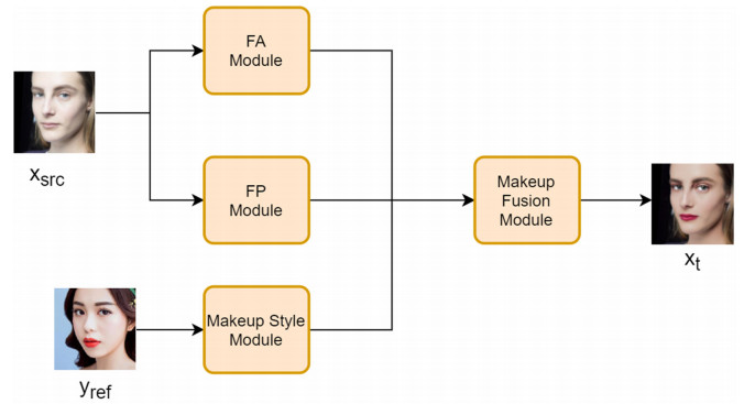
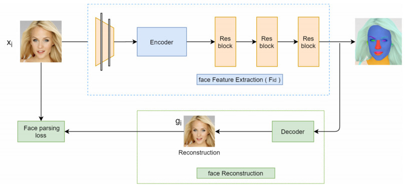
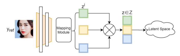
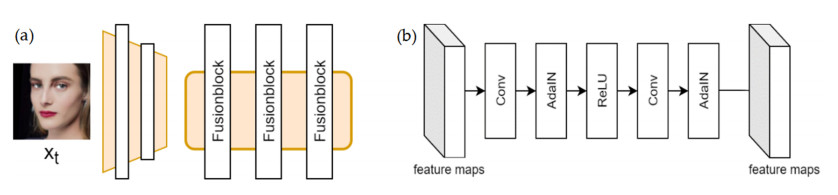
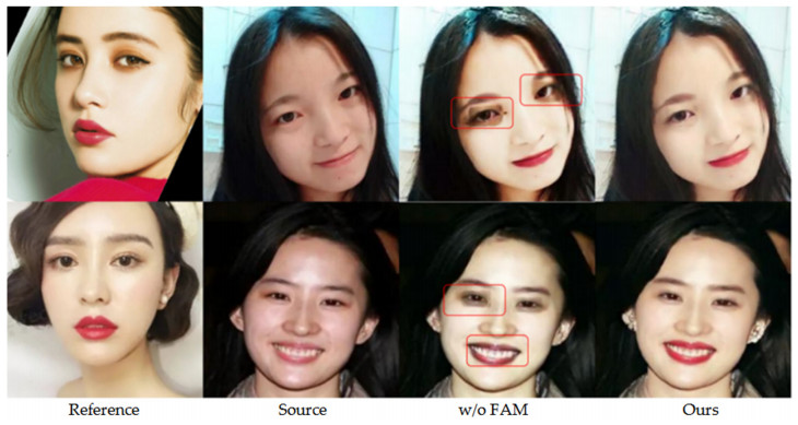
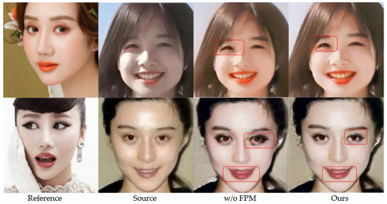
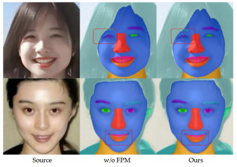
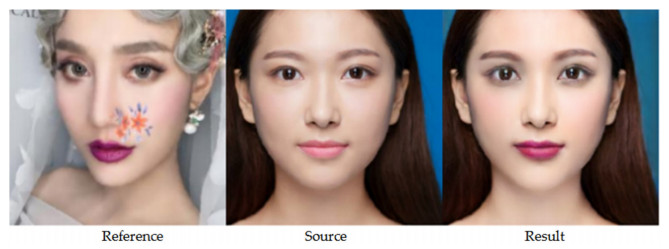
Facial makeup transfer is a special form of image style transfer. For the reference makeup image with large-pose, improving the quality of the image generated after makeup transfer is still a challenging problem worthy of discussion. In this paper, a large-pose makeup transfer algorithm based on generative adversarial network (GAN) is proposed. First, a face alignment module (FAM) is introduced to locate the key points, such as the eyes, mouth and skin. Secondly, a face parsing module (FPM) and face parsing losses are designed to analyze the source image and extract the face features. Then, the makeup style code is extracted from the reference image and the makeup transfer is completed through integrating facial features and makeup style code. Finally, a large-pose makeup transfer (LPMT) dataset is collected and constructed. Experiments are carried out on the traditional makeup transfer (MT) dataset and the new LPMT dataset. The results show that the image quality generated by the proposed method is better than that of the latest method for large-pose makeup transfer.

Keywords:

Citation: Qiming Li, Tongyue Tu. Large-pose facial makeup transfer based on generative adversarial network combined face alignment and face parsing[J]. Mathematical Biosciences and Engineering, 2023, 20(1): 737-757. doi: 10.3934/mbe.2023034

Related Papers:

[1]	Xin Zhou, Shangbo Zhou, Yuxiao Han, Shufang Zhu . Lévy flight-based inverse adaptive comprehensive learning particle swarm optimization. Mathematical Biosciences and Engineering, 2022, 19(5): 5241-5268. doi: 10.3934/mbe.2022246
[2]	Qing Wu, Chunjiang Zhang, Mengya Zhang, Fajun Yang, Liang Gao . A modified comprehensive learning particle swarm optimizer and its application in cylindricity error evaluation problem. Mathematical Biosciences and Engineering, 2019, 16(3): 1190-1209. doi: 10.3934/mbe.2019057
[3]	Xuepeng Zheng, Bin Nie, Jiandong Chen, Yuwen Du, Yuchao Zhang, Haike Jin . An improved particle swarm optimization combined with double-chaos search. Mathematical Biosciences and Engineering, 2023, 20(9): 15737-15764. doi: 10.3934/mbe.2023701
[4]	Yufei Wang, Yujun Zhang, Yuxin Yan, Juan Zhao, Zhengming Gao . An enhanced aquila optimization algorithm with velocity-aided global search mechanism and adaptive opposition-based learning. Mathematical Biosciences and Engineering, 2023, 20(4): 6422-6467. doi: 10.3934/mbe.2023278
[5]	Teng Fei, Hongjun Wang, Lanxue Liu, Liyi Zhang, Kangle Wu, Jianing Guo . Research on multi-strategy improved sparrow search optimization algorithm. Mathematical Biosciences and Engineering, 2023, 20(9): 17220-17241. doi: 10.3934/mbe.2023767
[6]	Hong Lu, Hongxiang Zhan, Tinghua Wang . A multi-strategy improved snake optimizer and its application to SVM parameter selection. Mathematical Biosciences and Engineering, 2024, 21(10): 7297-7336. doi: 10.3934/mbe.2024322
[7]	Shihong Yin, Qifang Luo, Yanlian Du, Yongquan Zhou . DTSMA: Dominant Swarm with Adaptive T-distribution Mutation-based Slime Mould Algorithm. Mathematical Biosciences and Engineering, 2022, 19(3): 2240-2285. doi: 10.3934/mbe.2022105
[8]	Shuang Tan, Shangrui Zhao, Jinran Wu . QL-ADIFA: Hybrid optimization using Q-learning and an adaptive logarithmic spiral-levy firefly algorithm. Mathematical Biosciences and Engineering, 2023, 20(8): 13542-13561. doi: 10.3934/mbe.2023604
[9]	Xiangyang Ren, Shuai Chen, Kunyuan Wang, Juan Tan . Design and application of improved sparrow search algorithm based on sine cosine and firefly perturbation. Mathematical Biosciences and Engineering, 2022, 19(11): 11422-11452. doi: 10.3934/mbe.2022533
[10]	Dongning Chen, Jianchang Liu, Chengyu Yao, Ziwei Zhang, Xinwei Du . Multi-strategy improved salp swarm algorithm and its application in reliability optimization. Mathematical Biosciences and Engineering, 2022, 19(5): 5269-5292. doi: 10.3934/mbe.2022247

Abstract

1. Introduction

1.1. Background

Meta heuristic algorithms mainly seek optimal solutions by simulating natural phenomena. This kind of algorithm is often called the intelligent optimization algorithm. At present, algorithms of this type are needed in a large number of fields, such as engineering design problems^[1,2,3], machine learning and theoretical analysis^[4,5,6,7] and energy saving and environmental protection^[8,9,10]. Sometimes people need to know what size industrial parts to choose to minimize cost, how to place trash cans in the city to provide maximum convenience for pedestrians, and so on. These problems can be solved quickly with the help of optimization algorithms. Depending on the source of inspiration, some researchers divide them into four categories: Population-based methods, methods inspired by physical phenomena, evolution-based strategies and methods inspired by human activities^[11]. Population-based meta-heuristic algorithms explore the search space through a population containing multiple individuals. Each individual represents a potential solution, and these individuals generate new solutions through different update ways. Through several iterations, the agents in the population gradually converge to the vicinity of the true solution. Inspired by natural selection, evolution-based meta-heuristic algorithms search for optimal solutions by simulating the evolutionary and genetic mechanisms of living organisms. The algorithm updates the individual through genetic operations, produces new solutions and selects better offspring. Physics-based metaheuristics update individuals by simulating physical laws and gradually approaching the true solution. Human-based metaheuristics are updating agents by imitating human behavior. Researchers have proposed many metaheuristic algorithms like this one by looking to nature for inspiration. They have the advantage of fast convergence and simple computation. However, excessive pursuit of convergence speed may lead to insufficient population diversity and premature convergence. Of course, these challenges are also the motivation for researchers to continuously explore and improve metaheuristic algorithms.

1.2. Literature review

The chicken swarm optimization (CSO) algorithm was initially proposed by Meng et al. ^[12] in 2014. Since then, numerous scholars have made enhancements and extensions to the algorithm, enabling its application across a broader range of disciplines. Inspired by the behavior of chickens, the CSO algorithm incorporates three different roles in the swarm: Roosters, hens and chicks. The rooster assumes an active role in food search within the flock while hens follow suit; meanwhile, chicks explore their surroundings for sustenance. Each colony can be divided into groups comprising one rooster alongside multiple hens and chicks. Different roosters adhere to varying locomotion rules with competition arising among them based on a specific hierarchical order. Aiming at the problem that the original CSO algorithm is easy to converge prematurely and fall into local optimum, many people have improved the update method of agents. To address this issue, Wu et al.^[13] introduced a new CSO that incorporates a portion of roosters' learning into the chicks' position update equation and introduces inertia weight and learning factor. As the most numerous individual in the population, the performance of CSO is greatly affected by how the hens update. Therefore, Chen et al.^[14] improved the update equation of hens.

The process of chicks following hens to find food is blind. Due to the lack of autonomy, the chicks are easily linked by the hens and, thus, fall into local optima. To solve this problem, Wang et al.^[15] proposed to introduce a mutation strategy for chicks to enhance the population diversity and help them get rid of the dilemma of falling into local optimum. The hens follow the lead rooster, while the chicks follow their mother for food. When the roosters get trapped in local optima, the hens and chicks will converge too early, reducing the effect of global optimization. Based on this problem, Verma et al. ^[16] introduced Levy's Flight strategy to solve the problems of local optimal and premature convergence. Ahmed et al.^[17] improved the search capability of CSO by applying logistic and tending to chaotic maps to help the CSO swarm to better explore the search space. Many researchers prefer to combine universal strategies such as Levy's flight and chaotic map with different swarm intelligence algorithms to improve the search effect of the algorithm. Other researchers have set their sights on improving these strategies. Recently, Yang et al.^[18] studied how to improve the probabilistic selection of chaotic operators based on the maximum Lyapunov exponent (MLE), and added this new multiple chaotic local operator to the slime mold algorithm (SMA) to achieve surprising results.

Aiming at the problem that the convergence speed of CSO algorithm is not satisfactory enough and difficulty in obtaining the global optimal solution of CSO, Wang et al.^[19] proposed an adaptive CSO algorithm with fuzzy strategy (FCSO). In the FCSO algorithm, the fuzzy system and cosine function are integrated into the CSO algorithm simultaneously. The fusion of optimization algorithms with machine learning techniques represents a widely explored area of research. Moldovan ^[20], for instance, leveraged the CSO algorithm to enhance the performance of the support vector machine (SVM) through hyperparameter optimization. This approach aims to achieve improved classification accuracy and showcases the growing synergy between optimization techniques and machine learning methods. In 2018, Mohamed ^[21] mapped real number vectors to integer space and used modified CSO to improve the performance of the greedy algorithm, which achieved good results. In addition to, some scholars have combined CSO with other swarm intelligence optimization algorithms or evolutionary algorithms to make up for some shortcomings of CSO. Abbas et al.^[22] combined CSO and the bacterial foraging optimization (BFA) algorithm, and this hybrid technique effectively reduced the computational cost and load. Torabi and Safi-Esfahani ^[23] combined CSO with the raven roosting optimization (RRO) algorithm to achieve a better transition between local exploitation and global exploration. Deb and Gao ^[24] combined CSO and the ant lion optimization algorithm (ALO) ^[25] to deal with the charger distribution problem, and the combination of CSO and ALO can improve the accuracy of CSO, thus preventing it from falling into local optimum. Deb et al. ^[26] also proposed the synergy of CSO with a new teaching-learning-based optimization (TLBO) algorithm, and proposed a new constraint handling mechanism to improve CSO. In 2019, Zouache et al.^[27] successfully applied CSO to the field of multi-objective optimization. Since then, some scholars ^[28] have continuously improved multi-objective CSO to improve algorithm performance and applied it to a lot of fields.

As previously mentioned in the CSO algorithm, roosters exhibit the highest search capability and are succeeded by hens, the largest agent class in the population. Chicks rely on their mothers for foraging and lack independence. Roosters handle global exploration, while hens and chicks manage local exploitation. However, the algorithm's search accuracy is unsatisfactory, prone to falling into local optima. Two reasons contribute to these issues: The hen's search method is not optimal, leading to low accuracy and premature convergence, and chicks' reliance on their mothers for food results in a limited learning scope and insufficient autonomous search ability. Consequently, chicks prematurely converge under maternal influence, leading to local optima challenges. Addressing this urgent concern, the paper is dedicated to refining the search methods for hens and chicks. It introduces a new CSO algorithm called chicken swarm optimization combining Pad $\acute{e}$ approximation, random learning and population reduction techniques (PRPCSO). The primary contributions of this study are outlined as follows:

1) A novel and efficient approach based on Pad $\acute{e}$ approximate technique is proposed to enhance the ability of the CSO algorithm in solving optimization problems. The fitting function used in this strategy is different from other linear approximation or quadratic approximation methods, but with the help of a complex nonlinear rational function, the extreme point is calculated from the mathematical point of view to approximate, which can significantly improve the solution accuracy and development ability of the CSO algorithm, and avoid local convergence.

2) Aiming at the problem that chicks are easy to fall into local optimum under the influence of their mother hens, a random learning mechanism is introduced. This mechanism has a special way of thinking when it comes to selecting random individuals. It selects from the same type of high-performing agents (i.e., chicks), rather than selecting them completely at random. This mechanism encourages chicks to follow their mother while learning from other good peers, preventing them from falling into local optima.

3) This study has developed a novel intelligent population size shrinking strategy. It not only considers adjusting the population size based on the number of fitness function calls but also creatively takes into account the variations in the obtained optimal solutions over the recent iterations. The strategy can eliminate bad and preserve good, prevent premature convergence, and reduce the amount of computation.

The rest of this paper is organized as follows. In Section 2, the CSO algorithm is briefly reviewed. Section 3 describes the main content and framework of PRPCSO. In Section 4, our proposed algorithm is tested with the other four famous, excellent algorithms on 23 test functions, and the experimental results are compared and analyzed. To investigate the application of PRPCSO to real problems, in Section 5, six real engineering design problems are described and analyzed experimentally. Finally, Section 6 contains the conclusions and perspectives of this work.

2. Mathematical model and basic knowledge

2.1. Principle of CSO algorithm

CSO is inspired by the foraging behavior of the flock and maps the behavior of the flock to mathematics. For simplicity, the behavior of the chicken is idealized according to the following rules.

1) A chicken swarm is divided into small groups. Each group has a rooster, many hens and chicks.

2) The role identification of chickens and the division of groups are realized according to their fitness values. Several chickens with the best fitness values are selected as roosters, and each rooster is used as the leader of a group. Except for a few chicks with the worst fitness values, the rest were identified as hens. The hens randomly select a group and randomly associates with some chicks in the group.

3) The hierarchy, dominance and mother-child relationships in the population are updated every few ( $G$ ) iterations.

4) The rooster acts as a leader in the search for food. Suppose chickens steal food randomly from each other. Chicks search for food near their mother (hens).

Suppose $rNum$ , $hNum$ , $cNum$ and $mNum$ correspond to the number of roosters, chickens, chickens and mother hens, respectively. For the problem of optimizing minimization, $rNum$ chickens with the lowest fitness value are assumed to be roosters, the worst $cNum$ chicken is considered to be chicks and the rest of the chickens are considered hens. $mNum$ chickens are randomly selected as mother hens in the hens swarm. All $N$ chickens are represented by their positions $x^t_{i, j}$ , ( $i \in [1, ..., N], j \in [1, ..., D]$ ) at time $t$ , looking for food in a search space.

2.2. The mathematics of CSO

Different members of the swarm move differently. Roosters search in the following way:

$\begin{equation} x^{t+1}_{i, j} = x^{t}_{i, j}(1+Randn(0, \sigma^{2})), \end{equation}$

(2.1)

$\begin{equation} \sigma^{2} = \begin{cases} 1, &if\; f_i\leq f_k\\exp(\frac{f_k-f_i}{\mid f_i \mid+\epsilon}), &otherwise \end{cases}, k\in [1, RN], k\neq i. \end{equation}$

(2.2)

Here $Randn(0, \sigma^{2})$ denotes a random number generated from a Gaussian distribution with mean zero and variance $\sigma^{2}$ . $k$ is the index of a rooster selected at random from the roosters and $f_k$ is its corresponding fitness value. $\epsilon$ is the smallest constant added to avoid a zero denominator.

Hens also compete with other chickens for food while following their mate roosters for food:

$\begin{equation} x^{t+1}_{i, j} = x^{t}_{i, j}+C_{1}Rand(x^t_{r1, j}-x^t_{i, j})+C_{2}Rand(x^t_{r2, j}-x^t_{i, j}), \end{equation}$

(2.3)

$\begin{equation} \begin{cases} C_{1} = exp(\frac{f_i-f_{r1}}{\mid f_i \mid+\epsilon})\\C_{2} = exp(f_{r2}-f_i) \end{cases}, \end{equation}$

(2.4)

where $Rand$ is a random number generated from a uniform distribution obeying [0, 1], $r1$ is the index of the mate of this hen in the group and its corresponding fitness value is $f_{r1}$ . In addition, an individual randomly selected from the group of roosters and hens is $r2$ , whose fitness value is $f_{r2}$ . $C_{1}$ and $C_{2}$ represent the influence factors of the hen's mate and other hens on the focal hen.

The chicks are entirely dependent on the influence of their mother for locating food:

$\begin{equation} x^{t+1}_{i, j} = x^{t}_{i, j}+FL(x^t_{m, j}-x^t_{i, j}), \end{equation}$

(2.5)

where $m$ is the index of the mother hen that the chick follows and $x^t_{m, j}$ is the position of the mother hen of the $i$ th chick (i.e., the $m$ th hen) in the $j$ th dimension. $FL$ is a parameter chosen from [0, 2] that represents the influence factor of the mother hen's position on the position of this chick.

3. The proposed optimization algorithm

3.1. Pad $\acute{e}$ approximate strategy

In this section, the Pad $\acute{e}$ approximate technique is introduced in order to construct an efficient intelligent optimization algorithm. This is a local search strategy that swiftly identifies optimal points in the proximity of several agents through solving for extreme points in a rational function fitting manner. This strategy contributes to enhancing the precision and efficiency of the local search carried out by hens. The Pad $\acute{e}$ approximation approximates $f(x)$ by using the following rational function:

$\begin{equation} T(x)\simeq T_{[M, N]}(x) = \frac{P(x)}{Q(x)} = \frac{\sum\limits_{i = 0}^{M} p_{i}(x-x_{0})^{i}}{\sum\limits_{i = 0}^{N} q_{i}(x-x_{0})^{i}}, \end{equation}$

(3.1)

which the mathematical expression is a kind of Pad $\acute{e}$ approximation. The coefficients $p_{i}$ and $q_{i}$ are unique up to constant and are generally normalized as $q_{0} = 1$ . Pad $\acute{e}$ approximate technique is a powerful approximate method for approximating rational functions. One of the most important advantages is that it is not restricted to the radius of convergence of the Taylor expansion^[29]. Specifically, Pad $\acute{e}$ approximate has the best convergence performance when the numerator and denominator have equal or almost equal orders. Rational fractions can provide better approximations either within or outside the radius of convergence. This method is the backbone of asymptotic waveform evaluation^[30,31] and has also been widely used by researchers to calculate frequency responses in recent years due to its extremely high efficiency and accuracy. This is the inspiration for our use of rational functions instead of standard polynomials. Therefore, in this paper, Pad $\acute{e}$ approximate technique is used to help hens to locate excellent solutions more quickly and accurately, which improves the development ability and solution accuracy of the CSO algorithm. We consider using the following ^[2,1] Pad $\acute{e}$ approximation:

$\begin{equation} T(x) = \frac{a_{1}+a_{2}x^{2}}{1+a_{3}x}, \end{equation}$

(3.2)

where $a_{1}, a_{2}$ and $a_{3}$ are real parameters. Let $T(x)$ be the interpolation rational function of $f(x)$ at abscissae $x_{k}$ , $x_{k+1}$ , $x_{k+2}$ . That is,

$\begin{equation} \left\{ \begin{aligned} T(x_{k}) = \frac{a_{1}+a_{2}x_{k}^{2}}{1+a_{3}x_{k}} = f(x_{k})\; \; \; \; \; \; \; \; \\ T(x_{k+1}) = \frac{a_{1}+a_{2}x_{k+1}^{2}}{1+a_{3}x_{k+1}} = f(x_{k+1})\\ T(x_{k+2}) = \frac{a_{1}+a_{2}x_{k+2}^{2}}{1+a_{3}x_{k+2}} = f(x_{k+2}). \end{aligned} \right. \end{equation}$

(3.3)

According to Eq (3.3), it can be calculated that:

$\begin{equation} a_1 = \frac{(x_{k+2}-x_{k+1})f(x_{k+1})f(x_{k+2})x_{k}^2+(x_{k}-x_{k+2})f(x_{k})f(x_{k+2})x_{k+1}^2+(x_{k+1}-x_{k})f(x_{k})f(x_{k+1})x_{k+2}^2}{(f(x_{k+2})x_{k+2}-f(x_{k+1})x_{k+1})x_{k}^2+(f(x_{k})x_{k}-f(x_{k+2})x_{k+2})x_{k+1}^2+(f(x_{k+1})x_{k+1}-f(x_{k})x_{k})x_{k+2}^2}, \end{equation}$

(3.4)

$\begin{equation} a_2 = \frac{(x_{k}-x_{k+1})f(x_{k}) f(x_{k+1}) +( x_{k+2}- x_{k}) f(x_{k}) f(x_{k+2}) +( x_{k+1}- x_{k+2}) f(x_{k+1}) f(x_{k+2})}{(x_{k}^2-x_{k+1}^2)f(x_{k+2})x_{k+2}+(x_{k+2}^2-x_{k}^2)f(x_{k+1})x_{k+1}+(x_{k+1}^2-x_{k+2}^2)f(x_{k})x_{k}}, \end{equation}$

(3.5)

$\begin{equation} a_3 = \frac{(x_{k+2}^2-x_{k+1}^2)f(x_{k})+(x_{k}^2-x_{k+2}^2)f(x_{k+1})+(x_{k+1}^2-x_{k}^2)f(x_{k+2})}{(x_{k+1}^2-x_{k+2}^2)f(x_{k})x_{k}+(x_{k+2}^2-x_{k}^2)f(x_{k+1})x_{k+1}+(x_{k}^2-x_{k+1}^2)f(x_{k+2})x_{k+2}}. \end{equation}$

(3.6)

Combining the above formulas, the minimal of approximate curve $T(x)$ can be attained as follows:

$\begin{equation} x^{*} = -\frac{1}{a_{3}}\pm\sqrt{abs(\frac{1}{a_{3}^{2}}+\frac{a_{1}}{a_{2}})}. \end{equation}$

(3.7)

The Pad $\acute{e}$ approximate operator is a local search operator that uses a curve to fit the structure of a rational function to reach the extreme point of the curve. In the Eq (3.7), there are two solutions of $x^*$ , and here, the greedy idea is used to compare these two $x^*$ with the fitness value of the original hen to select the best one among the three kinds of hens. The whole process is embodied in , where the hen is first updated to get $x^{t+1}$ in the original CSO way with Eqs (2.3) and (2.4). Next, the Pad $\acute{e}$ approximate strategy is performed and three neighboring hens $x_k$ , $x_{k+1}$ , $x_{k+2}$ in the hen group are selected and the parameters $a_1$ , $a_2$ and $a_3$ are calculated based on the positions and fitness values of these three hens, shown in Eqs (3.4)–(3.6). $x^*$ is split into two solutions $H(k)$ and $h(k)$ . Finally, the best one among the three ( $H(k)$ , $h(k)$ and $x^{t+1}$ ) is selected as the output solution.

Algorithm 1: The second degree Pad $\acute{e}$ approximate strategy
Require: $x^t_{i, j}$
Ensure: $x^{t+1}_{i, j}$
1: Generate random number $Rand$
2: for each $i \in [rNum+1, rNum+hNum]$ do
3: Calculate $x^{t+1}_{i, j}$ and $fit(i)$ according to the Eqs (2.3) and (2.4)
4: end for
5: for each $i \in [rNum+1, rNum+hNum-2]$ do
6: Select two agents around $x_{i}$ : $x_{i+1}$ , $x_{i+2}$
7: Calculate $a_1$ , $a_2$ , $a_3$ according to the Eqs (3.4)–(3.6)
8: Calculate $H(i)=-\frac{1}{a_{3}}+\sqrt{abs(\frac{1}{a_{3}^{2}}+\frac{a_{1}}{a_{2}})}$ , $h(i)=-\frac{1}{a_{3}}-\sqrt{abs(\frac{1}{a_{3}^{2}}+\frac{a_{1}}{a_{2}})}$
9: Let $tag1$ = $fit(H(i))$ , $tag2$ = $fit(h(i))$
10: if $tag1 < tag2$ then
11: $tag$ = $tag1$ ; $H(i)$ = $H(i)$
12: else
13: $tag$ = $tag2$ ; $H(i)$ = $h(i)$
14: end if
15: end for
16: if $tag < fit(i+2)$ then
17: $x^{t+1}_{i+2, j}$ = $H(i)$ ; $fit(i) = tag$
18: end if
return $x^{t+1}_{i, j}$

| Show Table

DownLoad: CSV

The foraging capability of hens plays a crucial role in determining the search efficiency of the algorithm and directly influences the foraging efficiency of their offspring. Hence, integrating the Pad $\acute{e}$ approximation strategy can enhance the hen's food-finding ability, ultimately maximizing the overall performance of the algorithm.

3.2. Random learning strategy

Considering that the chicks' search for food was completely affected by its mother, it was difficult to escape the local optimal situation when the mother hens are in a local optimal, so this work incorporates a random learning strategy for the process of finding food for chicks. The objective of this strategy is to decrease the reliance of chicks on their mothers and enhance the diversity of the population. As chicks follow mother hens for food, they also get help from well-performing agents within the same class. This not only assists chicks in steering clear of local optima, but also ensures a progressive behavior in chicks.

$\begin{equation} k_1, k_2, k_3 = randperm(pop-(rNum+hNum+1), 3)+rNum+hNum+1, \end{equation}$

(3.8)

$\begin{equation} [\sim , k] = min(fit(k_1), fit(k_2), fit(k_3)), \end{equation}$

(3.9)

$\begin{equation} x^{t+1}_{i, j} = x^{t}_{i, j}+rand(x^t_{m, j}-x^t_{k, j}), \end{equation}$

(3.10)

where $k_1$ , $k_2$ and $k_3$ are three different random indexes. $\sim$ is a placeholder for the output parameter, meaning that the minimum value of $fit(k_i)$ is ignored; we only need to record the index $k$ of the minimum value. Compare the fitness values of the chickens corresponding to the three indexes and select the optimal chicken $x_k$ . The specific process can be seen in Algorithm 2.

Algorithm 2 Random learning strategy
Input: $x^t_{m, j}$ , $x^t_{i, j}$
Output: $x^{t+1}_{i, j}$
1: Generate random number $Rand$
2: $k=randperm(pop-(rNum+hNum+1), 3)$
3: $k=k+rNum+hNum+1$
4: $[\sim, k]=min(fit(k_1), fit(k_2), fit(k_3))$
5: for each $i \in [rNum+hNum+1, pop]$ do
6: Calculate $x^{t+1}_{i, j}$ and $fit(i)$ according to the Eq (3.10)
7: end for
return $x^{t+1}_{i, j}$

| Show Table

DownLoad: CSV

The random learning strategy can reduce the dependence of the chicks on their mothers. If the mother chickens are unfortunate enough to fall into the local optimum, this mechanism ensures that chicks still retain the ability to escape from local extrema. Choosing the most suitable individual from three random candidates for learning rather than following a purely random approach ensures that the chicks' actions progress effectively. In general, incorporating the random learning strategy can increase the diversity of the population and overcome premature convergence.

3.3. Intelligent population size shrinkage strategy

Several swarm intelligence optimization algorithms have a common problem; that is, in the later stage of iteration, the algorithm tends to converge, thus a large number of individuals participating in optimization is redundant for the algorithm. Many researchers consider dynamically adjusting the population size. For example, Yang et al.^[32] proposed a new search method called a three-phase search approach with dynamic population size (TPSDP) and added the idea of dynamic population size, which depends on the number of iterations. Based on this, we propose a new intelligent population size shrinkage strategy. It takes into account both the number of fitness function calls and the optimal solution over $r$ iterations. It endeavors to sustain a sizable population in the initial iterations, particularly when the algorithm's obtained optimal solution exhibits substantial fluctuations. Conversely, it diminishes the population size during later iterations when the algorithm's optimal solution shows minimal variability. This concept aims to safeguard the algorithm's optimization effectiveness while alleviating computational demands. The population size gradually decreases according to Eq (3.11).

$\begin{equation} \begin{split} &pop = \begin{cases} p_{max}-round[\frac{(p_{max}-p_{min})NFE}{MAXNFE*\Phi^{\iota}(F)+\epsilon}], if\quad NFE < MAXNFE*\Phi^{\iota}(F)\\ max{(pop, p_{min})}, else \end{cases} \end{split} \end{equation}$

(3.11)

$\begin{equation} \Phi(F) = \frac{max(F)-mean(F)}{max(F)-min(F)}. \end{equation}$

(3.12)

Here $p_{max}$ and $p_{min}$ are the preset population maximum and minimum population sizes, and $pop$ is the number of agents within the current population. $F$ is the set of optimal solutions obtained by the algorithm in the last $r$ iterations, $max(F)$ is the maximum value in the set $F$ , $min(F)$ is the minimum value in the set $F$ and $mean(F)$ is the average value of $F$ . $\Phi(F)$ evaluates the performance of the last $r$ iterations by looking at the information provided by the maximum, minimum and average value of $F$ and $\Phi(F)$ is a number belonging to the range between zero and one. The value of $\Phi(F)$ is small when the convergence of the last $r$ iterations is fast, the value of $\Phi(F)$ converges to one when the algorithm's optimization process tends to converge and $\iota$ is a parameter. $MAXNFE$ is the maximum number of fitness function evaluations and $NFE$ is the number of fitness function evaluations within the current number of iterations. $\epsilon$ is the smallest constant added to avoid a zero denominator. Clearly, at the early stage of the population iteration, the algorithm converges faster, the $NFE$ is smaller and the population size is reduced slowly, which is exactly what this study wants to achieve. When the algorithm reaches the late iteration, the $NFE$ value gets closer to $MAXNFE$ and the convergence rate of the algorithm slows down so that the population size approaches $p_{min}$ . This mechanism of intelligently adjusting the population size helps the algorithm to make a smooth transition between global exploration and local exploitation. Premature convergence is avoided and the computational burden is reduced. See Algorithm 3 for details.

Algorithm 3 Intelligent population size shrinkage strategy
Input: $t$ , $M$ , $NFE$ , $MAXNFE$ , $G$
Output: $pop$ , New population after updating the number and population relationship of chickens
1: if $mod(t+1, G)==1$ then
2: $F=fmin(t-5, t-1)$
3: Calculate $\Phi(F)$ according to the Eq (3.12)
4: if $NFE < MAXNFE\Phi^{\iota}(F)$ then*
5: Calculate $pop$ according to the Eq (3.11)
6: else
7: $pop=max{(pop, p_{min})}$
8: end if
9: end if
10: Update the number and population relationship of three types of chickens in a new population
return $pop$

| Show Table

DownLoad: CSV

Considering the unique population relationship updating mechanism of the CSO algorithm; that is, the population is disrupted and the order is restablished every $G$ generations, it is possible to have an error while the number of chickens decreases but the relationships between them do not change. The population size shrinkage strategy is combined with the population relationship updating mechanism, then the population size is updated every $G$ generations. After that, the chicken families are redistributed to the new group to avoid the mismatch between the number of chickens and the relationship. Since the last $r$ optimal solutions are needed in the population size reduction strategy, the population size reduction strategy and the population relationship updating mechanism are applied when $mod(t+1, G) = = 1$ after the optimal solution is found in the $t$ th iteration.

Because the identity of the chickens and the relationship between them in the CSO algorithm are judged by the fitness value, the worst individuals can be naturally deleted after the implementation of the intelligent population size shrinkage strategy so that the excellent individuals can be retained. Reducing the population size helps to avoid getting stuck in a local optimum as well as reduce the computational effort of the algorithm. This process does not affect the accuracy of the algorithm because the poor performing chickens are removed.

How to balance exploration and exploitation is a very important research content for swarm intelligence algorithms (SIA). Most SIA focus on global exploration in the early stage and focus on local exploitation in the later stage, but CSO is different from it. As mentioned earlier, in CSO, roosters are responsible for global exploration, while hens and chicks are exploited in the vicinity of their respective leaders, roosters and mother hens, respectively. In each iteration, these three types of chickens are searching for the optimal solution at the same time, so the global exploration and local exploitation of CSO are carried out simultaneously. The population size shrinkage strategy and the population relationship update mechanism are carried out simultaneously, so when the population size changes, the roles of chickens in the population will be reconstructed. In the new population, agents with strong search ability can still be selected to be responsible for global exploration, and agents with weak search ability are responsible for local exploitation. When the algorithm enters the later stage, the number of agents with strong ability (roosters) is greatly reduced, and the number of agents with weak search ability (hens and chicks) is also reduced, but the hens are still the most numerous roles in all agents. The proportion of agents responsible for global exploration and local exploitation has not changed, so the balance between exploitation and exploration can be maintained even when the number of agents decreases.

3.4. The framework of PRPCSO

The improvement in CSO is mainly reflected in three aspects. First, the Pad $\acute{e}$ approximate operator helps the hens seek the optimal solution faster. It helps the agents to quickly converge near the approximate true solution, so as to improve the accuracy and exploitation ability of the algorithm. Meanwhile, due to the unique connection between hens and chicks, it also partially helps chicks in the foraging process. Second, combination of random learning strategy can help the population to be more diverse and help chicks avoid falling into local optima. Finally, a new intelligent population size shrinkage strategy is proposed. When the algorithm shows a convergence trend in nearly $r$ iterations, the poor individuals in the population were deleted. These three strategies are combined to construct the PRPCSO of this work.

The implementation process of PRPCSO is described in . Initially, the population is initialized, then the ranks and individual relationships within the population are updated in the first iteration. The largest number of chickens in the population, referred to as "hens", is then updated using the Pad $\acute{e}$ approximate strategy outlined in . Because the chicks completely rely on their mother hens to find food, their position update method is combined with a random learning strategy to avoid falling into local optimum, as shown in . After updating the positions of all three types of chickens, fitness values for each individual are evaluated. Once a preset number of $G$ iterations has been completed, the population undergoes shuffling and poor-performing chickens are removed based on the population size shrinkage strategy mentioned in Algorithm 3. This process creates a new order and individual relationships within the population. The iteration continues until termination conditions are met and outputs global optimal solution.

Algorithm 4 Pseudo code of the PRPCSO algorithm
Input: $FitFunc$ , $M$ , $pop$ , $p_{min}$ , $dim$ , $lb$ , $ub$ , $rPercent$ , $hPercent$ , $mPercent$
Output: Global best solution, Respective position vector
1: Initialize pop chickens and enter the relevant parameters;
2: All chickens were evaluated;
3: while $t < M$ do
4: if $t$ == 1 then
5: Rank according to fitness values to establish order as well as individual relationships within the group;
6: end if
7: for each $i \in [1, pop]$ do
8: if $i == rooster$ then
9: Update its location using Eqs (2.1) and (2.2);
10: else
11: if $i == hen$ then
12: Update its location by Algorithm 1;
13: else
14: Update its location by Algorithm 2;
15: end if
16: end if
17: Evaluate the new solution;
18: end for
19: if $mod(t+1, G)==1$ then
20: Generate new populations and update chickens' hierarchal order;
21: end if
22: end while
return Global best solution, Respective position vector

| Show Table

DownLoad: CSV

4. Experimental Study Ⅰ: Solving benchmark functions

4.1. Experimental preparation

To evaluate the robustness of PRPCSO, it was compared with six excellent algorithms on test functions and some engineering problems, they are CSO, grey wolf optimizer (GWO)^[33], sine cosine algorithm (SCA)^[34], ALO^[25], salp swarm algorithm (SSA)^[35], moth-flame optimization (MFO)^[36]. All experiments were run on MATLAB (R2021b). The portable computer used in this work is 12th Gen Intel (R) Core (trademark) i7-12700 (20 central processing units) with @2.10 Giga Hertz. Windows 10 operating system. All algorithms are compared after running 30 times with an initial population of 50 and 1000 iterations. All experiments were performed with the same settings. Finally, the performance metrics of 30 runs on the benchmark functions are obtained, which are the mean, standard deviation (std), minimum and maximum values of various benchmark functions, which are given in Tables 6–8, respectively. In the table, the bold font is the optimal solution, and the underlined font represents the sub-optimal solution.

4.2. Complexity analysis

As mentioned before, $pop$ stands for the number of agents, $dim$ is the number of dimensions and $M$ is the maximum number of iterations. The computational complexity of the metaheuristic can be defined as: $O(pop\cdot dim\cdot M)$ . The computational complexity of PRPCSO is $O(pop\cdot dim + (2pop\cdot dim+pop+2)\cdot M +pop\cdot dim /G) \approx O(pop\cdot dim\cdot M)$ . Because it is shown in , it has only one inner loop, and the algorithm needs additional fitness evaluation for $H(i)$ and $h(i)$ only in the Pad $\acute{e}$ approximate part. To ensure fair and unbiased experiments, $pop$ , $dim$ and $M$ are kept the same for all algorithms in this paper.

4.3. Benchmark functions

This section verifies the search capability of PRPCSO through 23 classical test functions. PRPCSO is used to find the extrema of these 23 functions. These functions are classical problems used to test the robustness of the algorithm and they are of various types, which facilitates researchers to investigate the algorithm from different aspects.

Tables 1–3 show the details of the 23 functions, where F1 to F13 are high-dimensional problems and F14 to F23 are mixed multi-modal problems. Functions F1 to F7 are unimodal, F6 is a step function with a minimum and is discontinuous, and F7 is a quadratic function containing noise. The multi-modal functions are F8 to F13, whose number of locally optimal solutions grows exponentially with the dimensionality of the problem, and it has been pointed out in ^[38] that this type of problem seems to be the most difficult class of optimization algorithms. The last class is F14 to F23, which are low-dimensional and contain few locally optimal solutions.

Table 1. Information on the seven unimodal benchmark functions.

Functions	Dim	Range	$f_{min}$
$f_{1}(x)=\sum\limits_{i=1}^{n} x^2_i$	30	$[-100,100]^n$	0
$f_{2}(x)=\sum\limits_{i=1}^{n}\|x_i\|+\prod^n_{i=1}\|x_i\|$	30	$[-10, 10]^n$	0
$f_{3}(x)=\sum\limits_{i=1}^{n}(\sum\limits_{j-1}^{i}x_j)^2$	30	$[-100,100]^n$	0
$f_{4}(x)=max_{i}\{ \|x_i\|, 1\leqslant i \leqslant n \}$	30	$[-100,100]^n$	0
$f_{5}(x)=\sum\limits_{i=1}^{n-1}[100(x_{i+1}-x^2_{i})^2+(x_i-1)^2]$	30	$[-30, 30]^n$	0
$f_{6}(x)=\sum\limits_{i=1}^{n}([x_i+0.5])^2$	30	$[-100,100]^n$	0
$f_{7}(x)=\sum\limits_{i=1}^{n} ix^4_i+random[0, 1)$	30	$[-1.28, 1.28]^n$	0

| Show Table

DownLoad: CSV

Table 2. Information on six multimodal functions.

Functions	Dim	Range	$f_{min}$
$f_{8}(x)=\sum\limits_{i=1}^{n}-x_isin(\sqrt{\|x_i\|})$	30	$[-500,500]^n$	-12569.5
$f_{9}(x)=\sum\limits_{i=1}^{n}[x^2_i-10\cos(2\pi x_i)+10]$	30	$[-5.12, 5.12]^n$	0
$f_{10}(x)=-20\exp(-0.2\sqrt{\frac{1}{n}\sum\limits_{i=1}^{n}x^2_i})$	30	$[-32, 32]^n$	0
$-\exp(\frac{1}{n}\sum\limits_{i=1}^{n}\cos(2\pi x_i))+20+e$
$f_{11}(x)=\frac{1}{4000}\sum\limits_{i=1}^{n} x^2_i-\prod^n_{i=1}\cos(\frac{x_i}{\sqrt{(i)}})+1$	30	$[-600,600]^n$	0
$f_{12}(x)=\frac{\pi}{n}\{10\sin(\pi y_1)+\sum\limits_{i=1}^{n-1}(y_i-1)^2[1+10\sin^2(\pi y_{i+1})]$	30	$[-50, 50]^n$	0
$+(y_n-1)^2\}+\sum\limits_{i=1}^{n}u(x_i, 10,100, 4)$
$y_i=1+\frac{x_i+1}{4}$
$u(x_i, a, k, m)=\begin{cases} k(x_i-a)^m \qquad x_i > a\\0 \qquad -a < x_i < a\\k(-x_i-a)^m \qquad x_i < -a \end{cases}$
$f_{13}(x)=0.1\{\sin^2(3\pi x_i)+\sum\limits_{i=1}^{n}x_i-1)^2[1+\sin^2(3\pi x_i+1)]$	30	$[-50, 50]^n$	0
$+(x_n-1)^2[1+\sin^2(2\pi x_n)]\}+\sum\limits_{i=1}^{n}u(x_i, 5,100, 4)$

| Show Table

DownLoad: CSV

Table 3. Fixed-dimension Multi-modal benchmark functions.

Functions	Dim	Range	$f_{min}$
$f_{14}(x)=(\frac{1}{500}+\sum\limits_{j=1}^{25}\frac{1}{j+\sum\limits_{i=1}^{2} (x_i-a_{ij})^6})^{-1}$	2	$[-65.536, 65.536]^n$	1
$f_{15}(x)=\sum\limits_{i=1}^{11}[a_i-\frac{x_1(b^2_i+b_1x_2)}{b^2_i+b_1x_3+x_4}]^2$	4	$[-5, 5]^n$	0.0003075
$f_{16}(x)=4x_1^2-2.1x^4_1+\frac{1}{3}x^6_3+x_1x_2-4x_2^2+4x_2^4$	2	$[-5, 5]^n$	-1.0316285
$f_{17}(x)=(x_2-\frac{5.1}{4\pi ^2}x^2_1+\frac{5}{\pi}x_1-6)^2$	2	$[-5, 5]^n$	0.398
$+10(1-\frac{1}{8\pi})\cos{x_1}+10$
$f_{18}(x)=[1+(x_1+x_2+1)^2(19-14x_1$	2	$[-2, 2]^n$	3
$+3x_1^2-14x_2+6x_1x_2+3x_2^2)]\times[30+(2x_1-3x_2)^2$
$\times (18-32x_1+12x_1^2+48x_2-36x_1x_2+27x_2^2)]$
$f_{19}(x)=\sum\limits_{i=1}^{4}c_i\exp (-\sum\limits_{j=1}^{3}a_{ij}(x_j-p_{ij})^2)$	4	$ ^[1,3]^n $	-3.86
$f_{20}(x)=\sum\limits_{i=1}^{4}c_i\exp (-\sum\limits_{j=1}^{6}a_{ij}(x_j-p_{ij})^2)$	6	$[0, 1]^n$	-3.32
$f_{21}(x)=\sum\limits_{i=1}^{5}[(X-a_i)(X-a_i)^T+c_i]^{-1}$	4	$[0, 10]^n$	-10
$f_{22}(x)=\sum\limits_{i=1}^{7}[(X-a_i)(X-a_i)^T+c_i]^{-1}$	4	$[0, 10]^n$	-10
$f_{23}(x)=\sum\limits_{i=1}^{10}[(X-a_i)(X-a_i)^T+c_i]^{-1}$	4	$[0, 10]^n$	-10

| Show Table

DownLoad: CSV

Table 1 corresponds to the mathematical representation of seven unimodal benchmark functions including function calculation formulas, dimension, the scope of the search space and the true optimal solution. Figure 3 is a schematic diagram on its 3D space, and it can be seen that the 3D plot of each function is concave and unimodal. Table 2 and Figure 4 correspond to the mathematical representation and 3D image presentation of the six multi-modal benchmark functions, respectively. It is obvious that the mathematical formulation of the multi-modal function is more complex than the mathematical formulation of the unimodel, and its multi-modal nature can be clearly seen from Figure 4. Finally, Table 3 and Figure 5 show fixed-dimension multi-modal benchmark functions, which have smaller dimension and search range than the other two, and the true optimal solution is also different from them.

Figure 1. The framework of CSO.

DownLoad: Full-Size Img PowerPoint

Figure 2. The framework of PRPCSO.

DownLoad: Full-Size Img PowerPoint

Figure 3. Unimodal benchmark functions.

DownLoad: Full-Size Img PowerPoint

Figure 4. Multi-modal benchmark functions.

DownLoad: Full-Size Img PowerPoint

Figure 5. Fixed-dimension Multi-modal benchmark functions.

DownLoad: Full-Size Img PowerPoint

4.4. Parameter setting

This section describes the parameter settings involved in the experiments. In order to ensure the fairness of the experiment, we only set the common parameters of all algorithms (such as population size, dimension of decision variable, maximum iteration number, etc.) without modifying the original code of the comparison algorithm. Other unique parameters will be configured in accordance with the settings outlined in the respective references of the algorithm. Moreover, specific parameters ( $\iota$ , $p_{min}$ , $r$ ) associated with PRPCSO require testing to ascertain their optimal values for the final configuration. For the parameter $MAXNFE$ , it is set to 200,000 in order to meet the requirements of the number of iterations; the other parameters of PRPCSO are kept consistent with the CSO algorithm.

During the experiment, four levels were considered for each parameter to be tested separately. Following the principles of the Taguchi method ^[37], 16 distinct value schemes were delimited. Considering that these three parameters all serve the population shrinkage strategy in order to reduce the running pressure of the algorithm, the average time of each run after running PRPCSO 30 times is taken as the response variable (consider the F1 test function), and the experimental results are detailed in Table 4.

Table 4. Parameter matrix and response variable values.

Index	$\iota$	$p_{min}$	$r$	response variable values
1	0.05	26	3	0.2488
2	0.05	28	5	0.2508
3	0.05	30	7	0.2517
4	0.05	32	9	0.3016
5	0.10	26	5	0.2416
6	0.10	28	3	0.2493
7	0.10	30	9	0.2500
8	0.10	32	7	0.2537
9	0.15	26	7	0.2458
10	0.15	30	3	0.2467
11	0.15	28	9	0.2474
12	0.15	32	5	0.2528
13	0.20	26	9	0.2377
14	0.20	32	3	0.2512
15	0.20	28	7	0.2444
16	0.20	30	5	0.2503

| Show Table

DownLoad: CSV

The average response variable values (ARV) corresponding to different levels of each parameter are shown in . The results indicate that the algorithm achieves optimal running speed when $\iota$ is set to 0.2, $p_{min}$ is set to 26 and $r$ is set to five.

Table 5. ARV for different parameter values.

$\iota$	ARV	$p_{min}$	ARV	$r$	ARV
0.05	0.2633	26	0.2435	3	0.2490
0.10	0.2487	28	0.2480	5	0.2488
0.15	0.2482	30	0.2497	7	0.2489
0.20	0.2459	32	0.2649	9	0.2592

| Show Table

DownLoad: CSV

4.5. Performance assessment

The test results of the PRPCSO algorithm and the other six algorithms on 23 benchmark functions are evaluated in this section. See Tables 6–8. The performance of each algorithm on these seven unimodal are provided in Table 6. The table results indicate GWO's strong competitiveness in addressing unimodal problems. However, PRPCSO still demonstrates commendable performance across five functions, excelling notably in functions F4 and F5, while securing the second-best performance in the remaining three functions (F1, F2, F7). The optimization problems in the F8 to F13 class are considered to be the most challenging. According to the performance analysis of these six problems in Table 7, it is not difficult to find that the performance of our proposed algorithm is significantly better than the other six comparison algorithms on F9–F12. In addition, the ranking of our proposed algorithm on F13 also shows strong competitiveness, which proves the superiority of PRPCSO in solving multimodal optimization problems. F14 to F23 are fixed-dimension multi-modal optimization problems. Table 8 shows that PRPCSO performs satisfactorily on 10 benchmark functions. Although other comparison algorithms also achieve similar optimal solutions, PRPCSO achieves lower std values with similar solutions. This proves that the superiority of PRPCSO is not only reflected in the solution accuracy but also in the solution robustness. In addition, PRPCSO shows better search ability than CSO on all test functions, which indicates that our proposed algorithm is an effective improvement.

Table 6. Results of unimodal benchmark functions.

function		CSO	GWO	SCA	ALO	SSA	MFO	PRPCSO
$f_{1}$	mean	3.52E-45	1.38E-69	2.27E-03	5.85E-07	8.83E-09	1333.3334	2.08E-46
	std	1.58E-44	3.79E-69	6.04E-03	4.17E-07	2.13E-09	3457.4590	4.40E-46
	min	9.09E-55	1.03E-72	8.13E-08	9.86E-08	5.07E-09	6.46E-06	9.23E-53
	max	8.52E-44	1.69E-68	2.45E-02	1.73E-06	1.40E-08	10000	2.12E-45
$f_{2}$	mean	8.00E-39	5.70E-41	1.00E-05	3.81E-01	0.5653	38.0002	2.69E-39
	std	1.75E-38	5.50E-41	1.86E-05	4.52E+01	0.8731	18.4578	4.69E-39
	min	1.70E-42	3.05E-42	4.97E-08	1.44E-02	0.0022	10.0001	5.84E-45
	max	7.89E-38	1.86E-40	7.65E-05	1.43E+02	3.8700	80.0000	1.95E-38
$f_{3}$	mean	2035.5631	3.72E-19	2860.8623	2.75E+02	41.8160	13459.6012	790.1403
	std	996.3636	1.54E-18	3010.3132	1.00E+02	29.3666	11102.5381	653.0734
	min	265.2085	2.32E-25	167.8583	8.25E+01	5.2595	142.0716	14.7509
	max	4489.5070	8.47E-18	11581.3715	5.24E+02	119.9813	35006.2993	2.73e+03
$f_{4}$	mean	8.8512	1.34E-17	13.21308	10.6803	4.2649	52.3683	2.98e-244
	std	8.6687	1.50E-17	7.2976	4.7471	3.2599	10.0618	0
	min	0.0053	1.11E-18	1.7985	4.0835	0.3896	25.0419	0
	max	26.3844	7.05E-17	29.5624	27.6545	12.2401	72.0400	8.94e-243
$f_{5}$	mean	34.2925	26.4411	86.190379	95.1932	131.0338	24484.8673	25.7341
	std	34.8687	0.6502	161.1930	189.8797	169.8673	40232.0860	0.6217
	min	26.9533	25.1891	28.0691	25.6544	24.9240	17.7747	24.6656
	max	218.8825	27.7481	647.0520	1044.0978	665.3988	90079.5694	27.2786
$f_{6}$	mean	3.0110	0.4261	4.291645	5.00E-07	8.98E-09	330.0084	0.0021
	std	0.5119	0.2772	0.3205	4.50E-07	1.49E-09	1807.5301	0.0015
	min	1.9506	0.000008	3.5429	7.13E-08	5.92E-09	9.19E-07	2.40e-04
	max	3.9455	1.253018	5.2019	1.72E-06	1.186E-08	9900.2500	0.0071
$f_{7}$	mean	0.016057	0.0003	0.0196	0.0437	0.0527	6.2370	0.0058
	std	0.0334	0.0002	0.0215	0.0189	0.0154	10.2140	0.0032
	min	0.0008	0.0000	0.0018	0.0120	0.0181	0.0262	0.0021
	max	0.1413	0.0008	0.1199	0.0891	0.0820	34.9651	0.0158

| Show Table

DownLoad: CSV

Table 7. Results of multi-modal benchmark functions.

function		CSO	GWO	SCA	ALO	SSA	MFO	PRPCSO
$f_{8}$	mean	-7654.4666	-6382.8472	-3926.4987	-5585.4462	-7754.1925	-8814.4881	-7424.1018
	std	562.7150	695.4723	266.1356	555.6855	587.7483	705.6383	706.8838
	min	-8659.9485	-8284.6623	-4434.8448	-8502.9480	-8891.6091	-10590.9578	-8525.7853
	max	-6868.3753	-4839.1327	-3424.6095	-5417.6748	-6783.2155	-7340.6252	-6075.9664
$f_{9}$	mean	0.7205	0.6116	19.4212	67.7566	47.7580	158.6928	0
	std	3.9465	1.9175	25.5091	19.8224	12.4763	33.1943	0
	min	0	0	3.00E-6	38.8033	18.9042	100.4905	0
	max	21.6160	7.2840	116.6615	117.4048	78.6015	238.0782	0
$f_{10}$	mean	6.93E-15	1.31E-14	10.6479	1.9030	1.8327	12.3331	6.09E-15
	std	1.86E-15	2.41E-15	9.3909	0.5052	0.7939	8.5879	1.80E-15
	min	4.44E-15	7.99E-15	0.0001	0.9329	2.15E-05	0.0010	4.44E-15
	max	7.99E-15	1.51E-14	20.3164	3.4621	3.2844	19.9591	7.99E-15
$f_{11}$	mean	0.0076	0.0014	0.1945	0.0121	0.0102	15.0656	0.0007
	std	0.0270	0.0055	0.2568	0.0123	0.0113	34.2321	0.0029
	min	0	0	2.00E-6	3.91E-05	1.82E-08	1.06E-05	0
	max	0.1156	0.0229	0.8175	0.0495	0.0394	90.7379	0.0136
$f_{12}$	mean	1.0635	0.0215	0.5964	8.8174	3.7450	8533334.23	0.0003
	std	2.3907	0.0131	0.2191	5.5645	2.5036	46738994.7573	0.0002
	min	0.1084	0.0057	0.3888	3.9331	0.1169	1.01E-05	3.79E-05
	max	9.0288	0.0654	1.4304	31.8536	12.9931	256000017.7553	0.0011
$f_{13}$	mean	3.7145	0.2961	6.6460	0.0147	0.0090	27337516.8500	0.0810
	std	11.3556	0.2001	9.4774	0.0268	0.0134	104036254.2859	0.0753
	min	0.9714	0.000016	2.0163	7.45E-08	4.06E-10	9.02E-06	0.0032
	max	63.8140	0.8582	40.0867	0.1316	0.0548	410062760.1113	0.3172

| Show Table

DownLoad: CSV

Table 8. Results of fixed-dimension multi-modal benchmark functions.

function		CSO	GWO	SCA	ALO	SSA	MFO	PRPCSO
$f_{14}$	mean	1.0641	1.0311	1.3949	1.2958	0.9980	1.4612	0.9980
	std	0.3622	4.0562	0.8071	0.6457	2.45E-16	0.7701	0
	min	0.9980	0.9980	0.9980	0.9980	0.9980	0.9980	0.9980
	max	2.9821	12.6705	2.9821	3.9683	0.9980	2.9821	0.9980
$f_{15}$	mean	0.0007	0.0050	0.0009	0.0048	0.0009	0.0015	0.0003
	std	0.0001	0.0085	0.0004	0.0125	0.0003	0.0036	0.0001
	min	0.0004	0.0003	0.0003	0005	0.0003	0.0006	0.0003
	max	0.0014	0.0203	0.0014	0.0632	0.0013	0.0204	0.0007
$f_{16}$	mean	-1.0316	-1.0316	-1.0316	-1.0316	-1.0316	-1.0316	-1.0316
	std	1.12E-10	2.98E-09	1.46E-05	4.00E-14	6.97E-15	6.77E-16	9.89E-11
	min	-1.0316	-1.0316	-1.0316	-1.0316	-1.0316	-1.0316	-1.0316
	max	-1.0316	-1.0316	-1.0315	-1.0316	-1.0316	-1.0316	-1.0316
$f_{17}$	mean	0.3978	0.3978	0.3987	0.3979	0.3979	0.3979	0.3979
	std	1.09e-07	5.43E-05	1.25E-03	4.67E-15	2.16E-15	0	0
	min	0.3978	0.3978	0.3979	0.3979	0.3979	0.3979	0.3979
	max	0.3978	0.3981	0.4029	0.3979	0.3979	0.3979	0.3979
$f_{18}$	mean	3	3.000005	3.000009	3	3	3	3
	std	2.17E-07	5.90E-06	1.84E-05	2.12E-13	7.82E-14	1.61E-15	9.99E-16
	min	3	3	3	3	3	3	3
	max	3	3	3.0001	3	3	3	3
$f_{19}$	mean	-3.8626	-3.8617	-3.8564	-3.8628	-3.8628	-3.8628	-3.8628
	std	6.25E-04	2.64E-03	3.12E-03	8.22E-15	8.42E-15	2.71E-15	2.71E-15
	min	-3.8627	-3.8627	-3.8625	-3.8628	-3.8628	-3.8628	-3.8628
	max	-3.8593	-3.8549	-3.8539	-3.8628	-3.8628	-3.8628	-3.8628
$f_{20}$	mean	-3.2680	-3.2679	-2.8998	-3.2507	-3.2382	-3.2203	-3.2780
	std	0.0660	0.0710	0.3329	0.0592	0.0558	0.0553	0.0543
	min	-3.3219	-3.3219	-3.2762	-3.3220	-3.3220	-3.3220	-3.3220
	max	-3.1459	-3.0866	-1.9181	-3.2031	-3.2008	-3.1376	-3.2031
$f_{21}$	mean	-9.8521	-9.3093	-2.8795	-7.3794	-7.9735	-7.1354	-10.1328
	std	0.9466	1.9185	2.2051	3.1235	3.2141	3.1857	0.0819
	min	-10.1531	-10.1531	-7.2573	-10.1532	-10.1532	-10.1532	-10.1532
	max	-5.0551	-5.0551	-0.497295	-2.6305	-2.6305	-2.6305	-9.7140
$f_{22}$	mean	-9.6777	-10.2254	-4.3896	-8.1360	-9.0111	-8.2851	-10.0877
	std	2.0425	0.9703	1.7626	3.0961	2.6190	3.3173	0.0824
	min	-10.4029	-10.4028	-6.8765	-10.4029	-10.4029	-10.4029	-10.4029
	max	-2.7658	-5.0876	-0.9079	-2.7519	-2.7519	-2.7659	-9.9515
$f_{23}$	mean	-10.2385	-10.2656	-4.881734	-7.4026	-9.3903	-8.3420	-10.0627
	std	2.7342	1.4814	1.6310	3.2671	2.6545	3.1846	1.4805
	min	-10.5364	-10.5363	-8.9339	-10.5364	-10.5364	-10.5364	-10.5364
	max	-2.8659	-2.4217	-0.9432	-2.8066	-2.4773	-2.4273	-3.8354

| Show Table

DownLoad: CSV

Unimodal functions can be used to evaluate the exploitation ability of an algorithm, and multi-modal functions can be used to evaluate the exploration ability of an algorithm. The ability of the algorithm to avoid local optima can be evaluated by using a multi-modal function. The experimental performance of the PRPCSO algorithm on 23 functions shows that it is an excellent combination of local exploitation and global exploration.

4.6. Statistical analysis

The nonparametric Friedman test^[39] was used to evaluate algorithms and calculate the probability values (p-values). This statistical test is used for multiple comparisons to determine significant differences between algorithms, and the number of trials in this paper is 30. The Friedman statistic can be computed using the following formula:

$\begin{equation} \chi^2_{F} = \frac{12N}{k(k+1)}[\sum\limits^k_{j = 1}r^2_j-\frac{k(k+1)^2}{4}]. \end{equation}$

(4.1)

In this work, $N$ and $k$ represent the number of datasets and algorithms, respectively, which are 23 and five; $r_j$ denotes the average ranking of $j_{th}$ algorithm. If the p-value is below a preset significance level (0.05 in this work), the null hypothesis is rejected and a statistically noteworthy distinction in the performance of each algorithm can be confirmed.

displays the outcomes of the test, where our proposed algorithm PRPCSO has the highest average rank on 14 test functions and, in addition, achieves sub-optimal average rank on four functions (F1, F7, F22, F23). The p-values were all $\le 0.05$ and the null hypothesis was rejected. The advantages of PRPCSO over other algorithms are proved. In addition, the Friedman test is performed on the ranking of these seven algorithms over 23 functions, and the overall mean ranks obtained are shown in Figure 6. It is easy to find that PRPCSO ranks first, followed by GWO, SSA, CSO, MFO, ALO and SCA. PRPCSO demonstrates a strong performance, while SSA and GWO also exhibit notable competitiveness in the results.

Table 9. Mean ranks of tested algorithms and p-value from Friedman test for 23 benchmark function.

function	CSO	GWO	SCA	ALO	SSA	MFO	PRPCSO	p-value
$f_{1}$	2.6667	1	6.5667	5.0667	4	6.3667	2.3333	1.14E-34
$f_{2}$	2.3333	1.2667	4	6.1667	5.2000	6.6333	2.4000	2.66E-33
$f_{3}$	5.5667	1	5.3667	3.2667	2.0300	6.7667	4.0000	1.26E-32
$f_{4}$	4.4333	2	5.2667	4.6667	3.6333	7	1	3.00E-31
$f_{5}$	4.0000	2.6667	5.2333	4.5333	4.0667	6.2000	1.3000	1.52E-19
$f_{6}$	5.9667	4.5667	6.7000	2	1	3.8000	3.9667	1.88E-31
$f_{7}$	2.9667	1	3.8000	5.7333	5.5333	6.2000	2.7667	8.66E-28
$f_{8}$	2.5667	4.6000	6.9667	5.7667	2.5000	1.2667	4.3333	5.65E-31
$f_{9}$	1.9833	2.0667	4.2000	5.6667	5.1667	6.9333	1.9833	3.77E-34
$f_{10}$	1.5500	2.9500	5.9333	5.3000	4.9000	5.8667	1.5000	6.91E-30
$f_{11}$	2.5000	2.3833	5.5667	5	4.9000	5.7000	1.9500	1.48E-21
$f_{12}$	4.8333	2.4000	4.4667	6.6667	5.7000	2.5667	1.3667	1.18E-28
$f_{13}$	6.1667	4.7667	6.7667	2.2667	1.7333	2.6667	3.6333	2.26E-29
$f_{14}$	3.2000	6.1667	5.9000	4.4167	3.3667	3.3667	1.5833	2.06E-20
$f_{15}$	4.0333	3.0333	5.3667	4.3333	4.8333	5.3333	1.0667	3.11E-17
$f_{16}$	2.2667	5.9667	7	4.7000	4.1667	1.9500	1.9500	3.24E-34
$f_{17}$	2.5333	6.0333	6.9667	3.5833	3.7167	2.5333	2.5333	7.98E-32
$f_{18}$	2.2333	6.4667	6.5333	4.5667	4.3333	2.1833	1.6833	7.23E-33
$f_{19}$	5.1333	5.6333	6.9333	3.5833	3.6167	1.5500	1.5500	9.02E-33
$f_{20}$	3.7000	3.6667	7	3.1000	5.0667	3.4833	1.9833	2.72E-19
$f_{21}$	4.5667	3.7000	6.1333	4.7333	3.1333	3.4833	2.2500	2.10E-11
$f_{22}$	5.3333	4.2667	6.3667	4	2.5000	2.8000	2.7333	1.43E-15
$f_{23}$	5.3333	4.4667	6.2333	4.2333	3.3333	2.0667	2.3333	2.90E-17

| Show Table

DownLoad: CSV

Figure 6. Rank of multiple algorithms on 23 functions.

DownLoad: Full-Size Img PowerPoint

After the above experimental analysis of 23 test functions, it can be concluded that compared with CSO, PRPCSO has greatly improved the solution accuracy and robustness in single-modal, multi-modal and mixed-dimensional multi-modal problems. This is due to the integration of multiple strategies: First, the Pad $\acute{e}$ approximation strategy helps hens to locate the optimal solution more quickly and accurately, and also improves the solving ability of chicks. This strategy helps the algorithm to exploit better locally. Second, the random learning mechanism is also very effective to help the chicks, which largely avoids the agents from falling into the dilemma of local optimum. In addition, the population size shrinkage strategy not only improves the running speed, but also ensures the balance between global exploration and local exploitation.

5. Experimental Study Ⅱ: Solving engineering problems

Benchmark function tests underscore the superior performance of PRPCSO in various straightforward problems. Nevertheless, real-world optimization challenges in diverse fields tend to be more intricate than benchmark functions, often involving complex computational methods and constraints. Consequently, there is a need to assess the effectiveness of PRPCSO in addressing real-world problems. Six practical engineering problems are first introduced (schematics from^[40,41]) in this section. PRPCSO is tested and compared with the other six excellent comparison algorithms (CSO, GWO, SCA, ALO, SSA and MFO) on these practical engineering design problems. These are the questions: Three-bar truss design, vessel design, rolling element bearing design, tension/compression spring design, cantilever beam design and gear train design. The engineering optimization problems pose significant challenges due to the presence of numerous intricate constraints in the solving process.

5.1. Three bar truss design problem

The first question concerns the design of the three-bar truss. The weight of the truss is minimized by adjusting the element parameters $s_1$ and $s_2$ . While the objective function is straightforward, the complexity arises from three types of constraints, namely, $G_1$ , $G_2$ and $G_3$ , corresponding to stress, deflection and buckling constraints, respectively. The mathematical formulation of the question is provided below and Figure 7 illustrates the schematic diagram:

$\begin{equation} min f(s) = (2\sqrt{2}s_1+s_2)\times V, \end{equation}$

(5.1)

$\begin{align} s.t.\quad &G_1 = \frac{\sqrt{2}s_1+s_2}{\sqrt{2}s^2_1+2s_1s_2}Q-\sigma \le 0, \\ &G_2 = \frac{z_2}{\sqrt{2}s_1^2+2s_1s_2}Q-\sigma \le 0, \\ &G_3 = \frac{1}{\sqrt{2}s_2+s_1}Q-\sigma \le 0, \end{align}$

(5.2)

where $s_1\in [0, 1], s_2\in [0, 1], V = 100 cm, Q = 2 KN/cm^2, \sigma = 2 KN/cm^2$ .

Figure 7. Three-bar truss design.

DownLoad: Full-Size Img PowerPoint

5.2. Pressure vessel design problem

The second problem wants to obtain the pressure vessel with the smallest possible manufacturing cost. The object function involves four variables ( $s_1, s_2, s_3, s_4$ ), and the optimization process is subject to four constraints ( $G_1, G_2, G_3, G_4$ ). The representation of the problem is depicted in Figure 8:

$\begin{equation} min f(s) = 0.6224s_1s_3s_4+1.7781s_2s_3^3+3.1661s_1^2s_4+19.84s_1^2s_3, \\ \end{equation}$

(5.3)

$\begin{align} s.t.\quad &G_1 = -s_1+0.0193s_3\le 0, \\ &G_2 = -s_2+0.00954s_3\le 0, \\ &G_3 = -\pi s^2_3s_4-\frac{4}{3}\pi s^3_3+1,296,000\le 0, \\ &G_4 = s_4-240\le 0, \end{align}$

(5.4)

where $s_1\in [0, 99]; s_2\in [0, 99]; s_3\in [0,200]; s_4\in [0,200]$ .

Figure 8. Pressure vessel design.

DownLoad: Full-Size Img PowerPoint

5.3. Rolling element bearing design problem

The objective of the third engineering case is to maximize the dynamic load carrying capacity of rolling element bearings. For computational convenience, the original objective function is transformed into a minimization optimization problem by $\times (-1)$ during the experimentation in this paper. The representation of this problem is shown in Figure 9:

$\begin{equation} \begin{split} &Variable\quad x = [d_m, d_b, Z, f_i, f_0, K_{d_{min}}, K_{d_{max}}, \epsilon , e, \xi], \\ &min f(x) = \begin{cases} f_c\cdot Z^{\frac{2}{3}}\cdot d_b^{1.8}\qquad if \quad d_b\le 25.4mm\\ 3.647f_c\cdot Z^{\frac{2}{3}}\cdot d_b^1.4 \qquad else \end{cases}, \end{split} \end{equation}$

(5.5)

$\begin{align} s.t., \quad &G_1(x) = \frac{\Phi _0}{2\sin^{-1}(\frac{d_b}{d_m})}-Z+1\ge 0, \\ &G_2(x) = 2d_b-K_{d_{min}}(d-D)\ge 0, \\ &G_3(x) = K_{d_{max}}(d-D)-2d_b\ge 0, \\ &G_4(x) = d_m-(0.5-e)(d+D)\ge 0, \\ &G_5(x) = (0.5+e)(d+D)-d_m\ge 0, \\ &G_6(x) = d_m-0.5(d+D)\ge 0, \\ &G_7(x) = 0.5(d-d_m-d_b)-\epsilon d_b\ge 0, \\ &G_8(x) = \zeta B_w-d_b\le 0, \\ &G_9(x) = f_i\ge 0.515, \\ &G_{10}(x) = f_0\ge 0.515, \end{align}$

(5.6)

where,

$\begin{align} &f_c = 37.91{1+[1.04(\frac{1-\gamma}{1+\gamma})^{1.72}(\frac{f_i(2f_0-1)}{f_0(2f_i-1)})^{0.4}]^{\frac{10}{3}}}^{-0.3}\times (\frac{\gamma^{0.3}(1-\gamma)^{1.39}}{f_0(1+\gamma)^{\frac{1}{3}}})(\frac{2f_i}{2f_i-1})^{0.41}, \end{align}$

$\begin{align} &\gamma = \frac{d_b}{d_m}, \quad f_i = \frac{r_i}{d_b}, \quad f_0 = \frac{r_0}{d_b}, \end{align}$

$\begin{align} &\Phi_0 = 2\pi-2\cos^{-1}\frac{(\frac{d-D}{2}-\frac{3T}{4})^2+(\frac{d}{2}-\frac{T}{4}-d_b)^2-(\frac{D}{2}+\frac{T}{4})^2}{2(\frac{d-D}{2}-\frac{3T}{4})(\frac{d}{2}-\frac{T}{4}-d_b)}, \end{align}$

$\begin{align} &T = d-D-2d_b, \quad d = 160, \quad D = 90, \quad B_w = 30, \quad r_i = r_0 = 11.033, \end{align}$

(5.7)

with variable range

$\begin{align} &0.5(d+D)\le d_m\le 0.6(d+D), \\ &0.15(d-D)\le d_b\le 0.45(d-D), \\ &4\le Z\le 50, \\ &0.515\le f_i\le 0.60, \\ &0.515\le f_0\le 0.60, \\ &0.40\le K_{d_{Min}}\le 0.50, \\ &0.60\le K_{d_{Max}}\le 0.70, \\ &0.30\le \epsilon \le 0.40, \\ &0.02\le e\le 0.10, \\ &0.60\le \zeta \le 0.85. \end{align}$

(5.8)

Figure 9. Rolling element bearing design.

DownLoad: Full-Size Img PowerPoint

5.4. Tension or compression spring design problem

This problem focuses on minimizing the coil weight by adjusting the variables $x_1, x_2, x_3$ , while ensuring satisfaction of four constraints. The problem is formulated as follows and the representation is shown in Figure 10:

$\begin{equation} \begin{split} &min f(X) = (x_3+2)x_2x_1^2, \end{split} \end{equation}$

(5.9)

$\begin{equation} \begin{split} &X = [x_1\quad x_2\quad x_3] = [d\quad D\quad N], \end{split} \end{equation}$

(5.10)

$\begin{align} s.t.\quad &G_1(x) = 1-\frac{x^3_2x_3}{71785x^4_1}\le 0, \\ &G_2(x) = \frac{4x^2_2-x_1x_2}{12566(x_2x_1^3-x^4_1)}+\frac{1}{5108x_1^2}\le 0, \\ &G_3(x) = 1-\frac{140.45x_1}{x^2_2x_3}\le 0, \\ &G_4(x) = \frac{x_1+x_2}{1.5}-1\le 0, \end{align}$

(5.11)

with variable range

$\begin{align} &0.05\le x_1\le 2.00, \\ &0.25\le x_2\le 1.30, \\ &2.00\le x_3\le 15.00. \end{align}$

(5.12)

Figure 10. Tension or compression spring design.

DownLoad: Full-Size Img PowerPoint

5.5. Cantilever beam design problem

The objective is to minimize the weight of the cantilever while adhering to constraints imposed by five distinct block lengths. The problem is formulated as follows and the representation is shown in Figure 11:

$\begin{equation} \begin{split} &min f(X) = 0.0624\times (x_1+x_2+x_3+x_4+x_5)\times L, \end{split} \end{equation}$

(5.13)

$\begin{align} s.t., \quad g_1(X) = \frac{61}{x^3_1}+\frac{37}{x^3_2}+\frac{19}{x^3_3}+\frac{7}{x^3_4}+\frac{1}{x^3_5}-1\le0, \end{align}$

(5.14)

with variable range

$\begin{align} 0.01\le x_i \le 100, i = (1, 2, ..., 5). \end{align}$

(5.15)

Figure 11. Cantilever beam design.

DownLoad: Full-Size Img PowerPoint

5.6. Gear train design problem

This question focuses on designing a gear train with the goal of minimizing the cost associated with the gear ratios. The problem has four integer variables where $T_a$ , $T_b$ , $T_d$ and $T_f$ denote the number of teeth of different gears. $\frac {T_b}{T_a}\times \frac{T_d}{T_f}$ is ratio of transmission. The equation of the problem is given below, as shown in Figure 12:

$\begin{equation} \begin{split} &min f(X) = (\frac{1}{6.931}-\frac{x_3x_2}{x_1x_4})^2, \end{split} \end{equation}$

(5.16)

$\begin{equation} \begin{split} &X = [x_1\quad x_2\quad x_3\quad x_4] = [T_a\quad T_b\quad T_d\quad T_f], \end{split} \end{equation}$

(5.17)

with variable range

$\begin{align} 12\le x_1, x_2, x_3, x_4\le 60. \end{align}$

(5.18)

Figure 12. Gear train design.

DownLoad: Full-Size Img PowerPoint

Table 10 presents the optimization results of seven swarm intelligence optimization algorithms applied to six real engineering problems. The findings demonstrate that our proposed algorithm, PRPCSO, exhibits superior performance across most engineering problems reflected in its consistently lowest average fitness values. While GWO outperforms PRPCSO in specific scenarios such as the pressure vessel design and rolling bearing element design problems, the proposed algorithm consistently secures the second-best solution with enhanced robustness. Notably, real-world optimization challenges often involve intricate constraints and diverse computational methods. The demonstrated accuracy and robust performance of PRPCSO in the aforementioned tests gives us greater confidence in it's ability to address complex optimization problems across various real-world domains.

Table 10. Comparison of results for classical engineering problems.

function		CSO	GWO	SCA	ALO	SSA	MFO	PRPCSO
Three-bar truss design	mean	263.929	263.898	264.625	263.896	263.895	263.916	263.896
	std	0.064	0.003	3.441	0.0003	0.001	0.039	6.09E-07
	min	263.896	263.896	263.902	263.896	263.896	263.896	263.896
	max	264.115	263.909	282.843	263.898	263.901	264.048	263.896
Pressure vessel design	mean	6685.481	6122.625	6866.114	484761.218	6607.671	6318.142	6369.648
	std	506.396	479.805	543.753	337653.799	604.644	528.172	330.952
	min	5939.799	5888.117	6194.835	36746.398	5919.239	5885.333	5936.837
	max	7339.426	7298.334	8531.817	1785286.904	7996.973	7319.001	7249.370
Rolling element bearing	mean	-83350.373	-85416.062	-81429.349	1.63E+21	-84461.8	-85180.2	-85413.231
design	std	2949.252	88.296	2546.690	1.15E+21	2090.336	610.748	219.026
	min	-85483.173	-85525.858	-84298.256	9.69E+18	-85538.930	-85549.239	-85549.239
	max	-71839.949	-85142.181	-74060.956	4.30E+21	-76489.035	-83233.128	-84521.638
Tension/compression	mean	0.013	0.013	0.013	1.73E+19	0.013	0.013	0.012
spring design	std	1.05E-07	5.87E-05	1.5E-04	2.79E+19	0.0001	0.001	0.0005
	min	1.267E-02	0.013	0.013	0.020	0.013	0.013	0.012
	max	0.018	0.013	0.013	9.67E+19	0.012	0.017	0.015
Cantilever beam design	mean	1.373	1.340	1.378	7.592	1.340	1.340	1.340
	std	0.029	3.54E-05	0.016	1.614	1.33E-05	0.0002	3.66E-05
	min	1.341	1.340	1.349	4.332	1.340	1.340	1.340
	max	1.434	1.340	1.406	11.055	1.340	1.341	1.340
Gear train design	mean	8.22E-11	1.25E-10	1.149E-09	0.001	1.63E-09	4.31E-09	6.31E-11
	std	2.38E-10	2.96E-10	1.03E-09	0.003	3.28E-09	6.63E-09	1.65E-10
	min	2.70E-12	2.70E-12	2.70E-12	1.48E-06	2.70E-12	9.93E-11	2.70E-12
	max	9.75E-10	9.92E-10	4.50E-09	0.013	1.83E-08	2.73E-08	8.89E-10

| Show Table

DownLoad: CSV

6. Summary and discussion

This paper proposed a new CSO algorithm (PRPCSO). First, a new approximate technique and the addition of the Pad $\acute{e}$ approximate operator effectively improved the accuracy of the algorithm. The random learning operator helped to reduce the possibility of chicks falling into local optima under the influence of their mother hens. Finally, the intelligent population size shrinkage strategy was used to eliminate some chickens with poor search capability in the later iteration of the algorithm, so as to boost the running speed of the algorithm and prevent premature convergence. At the same time, it ensured the balance between global exploration and local exploitation of the algorithm.

In order to evaluate the optimization ability of the algorithm, the PRPCSO algorithm was tested on two different experiments: Test functions and engineering problems. In Experiment I, 23 different types of functions were used to test the local exploitation and global exploration capabilities of the algorithm. Experimental results showed that PRPCSO algorithm has higher accuracy and stronger stability. The second set of experiments applied PRPCSO to practical engineering design, including six practical engineering design problems such as three-bar truss design, ship design, rolling bearing design, tension/compression spring design, cantilever beam design and gear train design. In addition, the high performance of PRPCSO in all experiments was verified by comparing six advanced optimization algorithms. The numerical results showed that the PRPCSO algorithm exhibits better stability and solution accuracy than CSO on all test problems. Among the seven algorithms, PRPCSO performed no worse than the other algorithms. In most cases, the results of PRPCSO were satisfactory. Therefore, PRPCSO can be considered as an effective improvement over the CSO algorithm. However, the experiments also showed some shortcomings of PRPCSO, mainly reflected in the processing of single-modal problems. GWO is a very competitive algorithm, which performed well on single-modal problems, while PRPCSO was at the second best level on partial problems. This is also one of the problems we need to solve in the future.

Although our improved algorithm performs well on 23 benchmark functions and six real-world engineering problems, there is no free lunch^[42], and no single algorithm performs good for all types of functions. Our proposed algorithm still has the potential to advance, so more research directions may be mined. Combining the strategy proposed in this work with other advanced metaheuristics algorithms (such as GWO, dung beetle optimizer etc.) may provide more satisfactory results. In the future, PRPCSO can find application in a broader spectrum of fields, including tasks like hyperparameter optimization for extreme learning machines or aiding in addressing issues within recommendation systems. Furthermore, there is potential for the development of multi-objective and many-objective versions of PRPCSO to tackle more intricate optimization problems.

Use of AI tools declaration

The authors declare they have not used Artificial Intelligence (AI) tools in the creation of this article.

Acknowledgments

This work has been supported by the Education Department of Jilin Province project (JJKH20220662KJ), National Natural Science Foundation of China (12026430) and Department of Science and Technology of Jilin Province project (20210101149JC, 20200403182SF).

Conflict of interests

The authors declare there is no conflict of interest.

References

[1]	W. S. Tong, C. K. Tang, M. S. Brown, Y. Q. Xu, Example-based cosmetic transfer, in 15th Pacific Conference on Computer Graphics and Applications (PG'07), (2007), 211-218. https://doi.org/10.1109/PG.2007.31
[2]	S. Liu, X. Ou, R. Qian, W. Wang, X. Cao, Makeup like a superstar: deep localized makeup transfer network, preprint, arXiv: 1604.07102.
[3]	D. Guo, T. Sim, Digital face makeup by example, in 2009 IEEE Conference on Computer Vision and Pattern Recognition, (2009), 73-79. https://doi.org/10.1109/CVPR.2009.5206833
[4]	L. Xu, Y. Du, Y. Zhang, An automatic framework for example-based virtual makeup, in 2013 IEEE International Conference on Image Processing, (2013), 3206-3210. https://doi.org/10.1109/ICIP.2013.6738660
[5]	C. Li, K. Zhou, S. Lin, Simulating makeup through physics-based manipulation of intrinsic image layers, in 2015 IEEE Conference on Computer Vision and Pattern Recognition (CVPR), (2015), 4621-4629. https://doi.org/10.1109/CVPR.2015.7299093
[6]	W. Xu, C. Long, R. Wang, G. Wang, DRB-GAN: A dynamic resblock generative adversarial network for artistic style transfer, in 2021 IEEE/CVF International Conference on Computer Vision (ICCV), (2021), 6383-6392. https://doi.org/10.1109/ICCV48922.2021.00632
[7]	H. Chen, L. Zhao, H. Zhang, Z. Wang, Z. Zuo, A. Li, et al., Diverse image style transfer via invertible cross-space mapping, in 2021 IEEE/CVF International Conference on Computer Vision (ICCV), (2021), 14860-14869. https://doi.org/10.1109/ICCV48922.2021.01461
[8]	Y. Hou, L. Zheng, Visualizing adapted knowledge in domain transfer, in 2021 IEEE/CVF Conference on Computer Vision and Pattern Recognition (CVPR), (2021), 13824-13833. https://doi.org/10.1109/CVPR46437.2021.01361
[9]	X. Zhang, Z. Cheng, X. Zhang, H. Liu, Posterior promoted GAN with distribution discrimi-nator for unsupervised image synthesis, in 2021 IEEE/CVF Conference on Computer Vision and Pattern Recognition (CVPR), (2021), 6519-6528. https://doi.org/10.1109/CVPR46437.2021.00645
[10]	P. Wang, Y. Li, N. Vasconcelos, Rethinking and improving the robustness of image style transfer, in 2021 IEEE/CVF Conference on Computer Vision and Pattern Recognition (CVPR), (2021), 124-133. https://doi.org/10.1109/CVPR46437.2021.00019
[11]	J. Y. Zhu, T. Park, P. Isola, A. A. Efros, Unpaired image-to-image translation using cycle-consistent adversarial networks, in 2017 IEEE International Conference on Computer Vision (ICCV), (2017), 2223-2232. https://doi.org/10.1109/ICCV.2017.244
[12]	H. Chang, J. Lu, F. Yu, A. Finkelstein, Pairedcyclegan: Asymmetric style transfer for applying and removing makeup, in 2018 IEEE/CVF Conference on Computer Vision and Pattern Recognition, (2018), 40-48. https://doi.org/10.1109/CVPR.2018.00012
[13]	H. J. Chen, K. M. Hui, S. Y. Wang, L. W. Tsao, H. H. Shuai, W. H. Cheng, Beautyglow: On-demand makeup transfer framework with reversible generative network, in 2019 IEEE/CVF Conference on Computer Vision and Pattern Recognition (CVPR), (2019), 10042-10050. https://doi.org/10.1109/CVPR.2019.01028
[14]	T. Li, R. Qian, C. Dong, S. Liu, Q. Yan, W. Zhu, et al., Beautygan: Instance-level facial makeup transfer with deep generative adversarial network, in Proceedings of the 26th ACM international conference on Multimedia, (2018), 645-653. https://doi.org/10.1145/3240508.3240618
[15]	T. Nguyen, A. T. Tran, M. Hoai, Lipstick ain't enough: beyond color matching for in-the-wild makeup transfer, in 2021 IEEE/CVF Conference on Computer Vision and Pattern Recognition (CVPR), (2021), 13305-13314. https://doi.org/10.1109/cvpr46437.2021.01310
[16]	Z. Sun, Y. Chen, S. Xiong, SSAT: A symmetric semantic-aware transformer network for makeup transfer and removal, in Proceedings of the AAAI Conference on Artificial Intelligence, 36 (2022), 2325-2334. https://doi.org/10.1609/aaai.v36i2.20131
[17]	Z. Huang, Z. Zheng, C. Yan, H. Xie, Y. Sun, J. Wang, et al., Real-world automatic makeup via identity preservation makeup net, in International Joint Conferences on Artificial Intelligence Organization, (2020), 652-658. https://doi.org/10.24963/ijcai.2020/91
[18]	Z. Wan, H. Chen, J. An, W. Jiang, C. Yao, J. Luo, et al., Facial attribute transformers for precise and robust makeup transfer, in 2022 IEEE/CVF Winter Conference on Applications of Computer Vision (WACV), (2022), 1717-1726. https://doi.org/10.1109/wacv51458.2022.00317
[19]	J. Lee, E. Kim, Y. Lee, D. Kim, J. Chang, J. Choo, Reference-based sketch image colorization using augmented-self reference and dense semantic correspondence, in 2020 IEEE/CVF Conference on Computer Vision and Pattern Recognition (CVPR), (2020), 5800–5809. https://doi.org/10.1109/cvpr42600.2020.00584
[20]	W. Jiang, S. Liu, C. Gao, J. Cao, R. He, J. Feng, et al., Psgan: Pose and expression robust spatial-aware gan for customizable makeup transfer, in 2020 IEEE/CVF Conference on Computer Vision and Pattern Recognition (CVPR), (2020), 5194–5202. https://doi.org/10.1109/CVPR42600.2020.00524
[21]	A. Vaswani, N. Shazeer, N. Parmar, J. Uszkoreit, L. Jones, A. N. Gomez, et al., Attention is all you need, in Advances in Neural Information Processing Systems, 30 (2017), 5998-6008.
[22]	H. Deng, C. Han, H. Cai, G. Han, S. He, Spatially-invariant style-codes controlled makeup transfer, in 2021 IEEE/CVF Conference on Computer Vision and Pattern Recognition (CVPR), (2021), 6549-6557. https://doi.org/10.1109/CVPR46437.2021.00648
[23]	K. Zhang, Z. Zhang, Z. Li, Y. Qiao, Joint face detection and alignment using multitask cascaded convolutional networks, IEEE Signal Process Lett., 23 (2016), 1499-1503. https://doi.org/10.1109/LSP.2016.2603342 doi: 10.1109/LSP.2016.2603342
[24]	Y. Wang, J. M. Solomon, Prnet: Self-supervised learning for partial-to-partial registration, in 33rd Conference on Neural Information Processing Systems (NeurIPS 2019), 32 (2019), 8812-8824. Available from: https://proceedings.neurips.cc/paper/2019/file/ebad33b3c9fa1d10327bb55f9e79e2f3-Paper.pdf.
[25]	K. Simonyan, A. Zisserman, Very deep convolutional networks for large-scale image recognition, preprint, arXiv: 1409.1556.
[26]	D. P. Kingma, P. Dhariwal, Glow: Generative flow with invertible 1x1 convolutions, in 32nd Conference on Neural Information Processing Systems (NeurIPS 2018), 31 (2018), 10236-10245. Available from: https://proceedings.neurips.cc/paper/2018/file/d139db6a236200b21cc7f752979132d0-Paper.pdf.
[27]	K. He, X. Zhang, S. Ren, J. Sun, Deep residual learning for image recognition, in 2016 IEEE Conference on Computer Vision and Pattern Recognition (CVPR), (2016), 770-778. https://doi.org/10.1109/CVPR.2016.90
[28]	C. Yu, J. Wang, C. Peng, C. Gao, G. Yu, N. Sang, Bisenet: Bilateral segmentation network for real-time semantic segmentation, in Computer Vision – ECCV 2018, 11217 (2018), 334-349. https://doi.org/10.1007/978-3-030-01261-8_20
[29]	T. Karras, S. Laine, T. Aila, A style-based generator architecture for generative adversarial networks, in 2019 IEEE/CVF Conference on Computer Vision and Pattern Recognition (CVPR), (2019), 4401-4410. https://doi.org/10.1109/CVPR.2019.00453
[30]	X. Huang, S. Belongie, Arbitrary style transfer in real-time with adaptive instance normalization, in 2017 IEEE International Conference on Computer Vision (ICCV), (2017), 1501-1510. https://doi.org/10.1109/ICCV.2017.167
[31]	I. Goodfellow, J. Pouget-Abadie, M. Mirza, B. Xu, D. Warde-Farley, S. Ozair, et al., Generative adversarial nets, in Proceedings of the 27th International Conference on Neural Information Processing Systems, 2 (2014), 2672–2680. https://dl.acm.org/doi/10.5555/2969033.2969125
[32]	J. Johnson, A. Alahi, L. Fei-Fei, Perceptual losses for real-time style transfer and super-resolution, in Computer Vision – ECCV 2016, 9906 (2016), 694-711. https://doi.org/10.1007/978-3-319-46475-6_43
[33]	D. P. Kingma, J. Ba, Adam: a method for stochastic optimization, preprint, arXiv: 1412.6980.
[34]	Y. Lyu, J. Dong, B. Peng, W. Wang, T. Tan, SOGAN: 3D-aware shadow and occlusion robust GAN for makeup transfer, in Proceedings of the 29th ACM International Conference on Multimedia, (2021), 3601-3609. https://doi.org/10.1145/3474085.3475531
[35]	J. Liao, Y. Yao, L. Yuan, G. Hua, S. B. Kang, Visual attribute transfer through deep image analogy, preprint, arXiv: 1705.01088.
[36]	Q. Gu, G. Wang, M. T. Chiu, Y. W. Tai, C. K. Tang, Ladn: Local adversarial disentangling network for facial makeup and de-makeup, in 2019 IEEE/CVF International Conference on Computer Vision (ICCV), (2019), 10481-10490. https://doi.org/10.1109/ICCV.2019.01058
[37]	B. Yan, Q. Lin, W. Tan, S. Zhou, Assessing eye aesthetics for automatic multi-reference eye in-painting, in 2020 IEEE/CVF Conference on Computer Vision and Pattern Recognition (CVPR), (2020), 13509-13517. https://doi.org/10.1109/CVPR42600.2020.01352

This article has been cited by:

Hussam N. Fakhouri, Faten Hamad, Abdelraouf Ishtaiwi, Amjad Hudaib, Niveen Halalsheh, Sandi N. Fakhouri, Advancing Engineering Solutions with Protozoa-Based Differential Evolution: A Hybrid Optimization Approach, 2025, 6, 2673-4052, 13, 10.3390/automation6020013

Reader Comments

Your name:*

Email:*
© 2023 the Author(s), licensee AIMS Press. This is an open access article distributed under the terms of the Creative Commons Attribution License (http://creativecommons.org/licenses/by/4.0)