We incorporate a practical data assimilation methodology into our previously established experimental-computational framework to predict the heterogeneous response of glioma cells receiving fractionated radiation treatment. Replicates of 9L and C6 glioma cells grown in 96-well plates were irradiated with six different fractionation schemes and imaged via time-resolved microscopy to yield 360- and 286-time courses for the 9L and C6 lines, respectively. These data were used to calibrate a biology-based mathematical model and then make predictions within two different scenarios. For Scenario 1, 70% of the time courses are fit to the model and the resulting parameter values are averaged. These average values, along with the initial cell number, initialize the model to predict the temporal evolution for each test time course (10% of the data). In Scenario 2, the predictions for the test cases are made with model parameters initially assigned from the training data, but then updated with new measurements every 24 hours via four versions of a data assimilation framework. We then compare the predictions made from Scenario 1 and the best version of Scenario 2 to the experimentally measured microscopy measurements using the concordance correlation coefficient (CCC). Across all fractionation schemes, Scenario 1 achieved a CCC value (mean ± standard deviation) of 0.845 ± 0.185 and 0.726 ± 0.195 for the 9L and C6 cell lines, respectively. For the best data assimilation version from Scenario 2 (validated with the last 20% of the data), the CCC values significantly increased to 0.954 ± 0.056 (p = 0.002) and 0.901 ± 0.061 (p = 8.9e-5) for the 9L and C6 cell lines, respectively. Thus, we have developed a data assimilation approach that incorporates an experimental-computational system to accurately predict the in vitro response of glioma cells to fractionated radiation therapy.
Citation: Junyan Liu, David A. Hormuth II, Jianchen Yang, Thomas E. Yankeelov. A data assimilation framework to predict the response of glioma cells to radiation[J]. Mathematical Biosciences and Engineering, 2023, 20(1): 318-336. doi: 10.3934/mbe.2023015
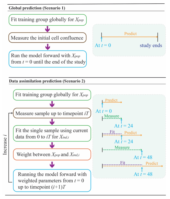
We incorporate a practical data assimilation methodology into our previously established experimental-computational framework to predict the heterogeneous response of glioma cells receiving fractionated radiation treatment. Replicates of 9L and C6 glioma cells grown in 96-well plates were irradiated with six different fractionation schemes and imaged via time-resolved microscopy to yield 360- and 286-time courses for the 9L and C6 lines, respectively. These data were used to calibrate a biology-based mathematical model and then make predictions within two different scenarios. For Scenario 1, 70% of the time courses are fit to the model and the resulting parameter values are averaged. These average values, along with the initial cell number, initialize the model to predict the temporal evolution for each test time course (10% of the data). In Scenario 2, the predictions for the test cases are made with model parameters initially assigned from the training data, but then updated with new measurements every 24 hours via four versions of a data assimilation framework. We then compare the predictions made from Scenario 1 and the best version of Scenario 2 to the experimentally measured microscopy measurements using the concordance correlation coefficient (CCC). Across all fractionation schemes, Scenario 1 achieved a CCC value (mean ± standard deviation) of 0.845 ± 0.185 and 0.726 ± 0.195 for the 9L and C6 cell lines, respectively. For the best data assimilation version from Scenario 2 (validated with the last 20% of the data), the CCC values significantly increased to 0.954 ± 0.056 (p = 0.002) and 0.901 ± 0.061 (p = 8.9e-5) for the 9L and C6 cell lines, respectively. Thus, we have developed a data assimilation approach that incorporates an experimental-computational system to accurately predict the in vitro response of glioma cells to fractionated radiation therapy.

| [1] | C. Fernandes, A. Costa, L. Osório, R. C. Lago, P. Linhares, B. Carvalho, et al., Current standards of care in glioblastoma therapy, in Glioblastoma, Codon Publications, (2017), 197–241. doi: 10.15586/codon.glioblastoma.2017.ch11 |
| [2] |
M. E. Davis. Glioblastoma: Overview of disease and treatment, Clin. J. Oncol. Nurs., 20 (2016), S2–S8. doi: 10.1188/16.CJON.S1.2-8 doi: 10.1188/16.CJON.S1.2-8

|
| [3] |
K. M. Walsh, H. Ohgaki, M. R. Wrensch, Chapter 1-Epidemiology, Handb. Clin. Neurol., 134 (2016), 3–18. doi: 10.1016/B978-0-12-802997-8.00001-3 doi: 10.1016/B978-0-12-802997-8.00001-3
|
| [4] |
C. Ke, K. Tran, Y. Chen, A. T. Di Donato, L. Yu, Y. Hu, et al., Linking differential radiation responses to glioma heterogeneity, Oncotarget, 5 (2014), 1657–1665. doi: 10.18632/oncotarget.1823 doi: 10.18632/oncotarget.1823
|
| [5] |
D. A. Jaffray, Image-guided radiotherapy: From current concept to future perspectives, Nat. Rev. Clin. Oncol., 9 (2012), 688–699. doi: 10.1038/nrclinonc.2012.194 doi: 10.1038/nrclinonc.2012.194
|
| [6] |
B. Wang, X. Zou, J. Zhu, Data assimilation and its applications, Proc. Natl. Acad. Sci. U.S.A., 97 (2000), 11143–11144. doi: 10.1073/pnas.97.21.11143 doi: 10.1073/pnas.97.21.11143
|
| [7] |
W. A. Lahoz, P. Schneider, Data assimilation: Making sense of earth observation, Front. Environ. Sci., 2 (2014), 16. doi: 10.3389/fenvs.2014.00016 doi: 10.3389/fenvs.2014.00016
|
| [8] |
M. Ghil, P. Malanotte-Rizzoli, Data assimilation in meteorology and oceanography, Adv. Geophys., 33 (1991), 141–266. doi: 10.1016/S0065-2687(08)60442-2 doi: 10.1016/S0065-2687(08)60442-2
|
| [9] | S. M. Bentzen, C. M. Joiner, The linear-quadratic approach in clinical practice, in Basic Clinical Radiobiology, CRC Press, (2009), 112–124. doi: 10.1201/9780429490606-10 |
| [10] |
D. A. Hormuth, A. M. Jarrett, E. A. B. F. Lima, M. T. McKenna, D. T. Fuentes, T. E. Yankeelov, Mechanism-based modeling of tumor growth and treatment response constrained by multiparametric imaging data, JCO Clin. Cancer Inf., 3 (2019), 1–10. doi: 10.1200/CCI.18.00055 doi: 10.1200/CCI.18.00055
|
| [11] |
D. A. Hormuth, M. Farhat, C. Christenson, B. Curl, C. Chad Quarles, C. Chung, et al., Opportunities for improving brain cancer treatment outcomes through imaging-based mathematical modeling of the delivery of radiotherapy and immunotherapy, Adv. Drug Deliv. Rev., 187 (2022), 114367. doi: 10.1016/j.addr.2022.114367 doi: 10.1016/j.addr.2022.114367
|
| [12] |
D. A. Hormuth, C. M. Phillips, C. Wu, E. A. B. F. Lima, G. Lorenzo, P. K. Jha, et al., Biologically-based mathematical modeling of tumor vasculature and angiogenesis via time-resolved imaging data, Cancers, 13 (2021), 3008. doi: 10.3390/cancers13123008 doi: 10.3390/cancers13123008
|
| [13] |
A. S. Kazerouni, M. Gadde, A. Gardner, D. A. Hormuth, A. M. Jarrett, K. E. Johnson, et al., Integrating quantitative assays with biologically based mathematical modeling for predictive oncology, Iscience, 23 (2020), 101807. doi: 10.1016/j.isci.2020.101807 doi: 10.1016/j.isci.2020.101807
|
| [14] |
R. C. Rockne, A. D. Trister, J. Jacobs, A. J. Hawkins-Daarud, M. L. Neal, K. Hendrickson, et al., A patient-specific computational model of hypoxia-modulated radiation resistance in glioblastoma using 18F-FMISO-PET, J. R. Soc. Interface., 12 (2015), 20141174. doi: 10.1098/rsif.2014.1174 doi: 10.1098/rsif.2014.1174
|
| [15] |
D. A. Hormuth, J. A. Weis, S. L. Barnes, M. I. Miga, V. Quaranta, T. E. Yankeelov, Biophysical modeling of in vivo glioma response after whole-brain radiation therapy in a murine model of brain cancer, Int. J. Radiat. Oncol. Biol. Phys., 100 (2018), 1270–1279. doi: 10.1016/j.ijrobp.2017.12.004 doi: 10.1016/j.ijrobp.2017.12.004
|
| [16] |
J. Liu, D. A. Hormuth, T. Davis, J. Yang, M. T. McKenna, A. M. Jarrett, et al., A time-resolved experimental-mathematical model for predicting the response of glioma cells to single-dose radiation therapy, Integr. Biol., 13 (2021), 167–183. doi: 10.1093/intbio/zyab010 doi: 10.1093/intbio/zyab010
|
| [17] |
S. Brüningk, G. Powathil, P. Ziegenhein, J. Ijaz, I. Rivens, S. Nill, et al., Combining radiation with hyperthermia: A multiscale model informed by in vitro experiments, J. R. Soc. Interface, 15 (2018), 20170681. doi: 10.1098/rsif.2017.0681 doi: 10.1098/rsif.2017.0681
|
| [18] |
E. J. Kostelich, Y. Kuang, J. M. McDaniel, N. Z. Moore, N. L. Martirosyan, M. C. Preul, Accurate state estimation from uncertain data and models: an application of data assimilation to mathematical models of human brain tumors, Biol. Direct., 6 (2011), 64. doi: 10.1186/1745-6150-6-64 doi: 10.1186/1745-6150-6-64
|
| [19] |
M. U. Zahid, N. Mohsin, A. S. R. Mohamed, J. J. Caudell, L. B. Harrison, C. D. Fuller, et al., Forecasting individual patient response to radiation therapy in head and neck cancer with a dynamic carrying capacity model, Int. J. Radiat. Oncol. Biol. Phys., 111 (2021), 693–704. doi: 10.1016/j.ijrobp.2021.05.132 doi: 10.1016/j.ijrobp.2021.05.132
|
| [20] | J. Liu, D. A. Hormuth, J. Yang, T. E. Yankeelov, A multi-compartment model of glioma response to fractionated radiation therapy parameterized via time-resolved microscopy data, Front. Oncol., 12 (2022), 811415. https://www.frontiersin.org/article/10.3389/fonc.2022.811415 |
| [21] |
Z. Neufeld, W. von Witt, D. Lakatos, J. Wang, B. Hegedus, A. Czirok, The role of Allee effect in modelling post resection recurrence of glioblastoma, PLoS Comput. Biol., 13 (2017), e1005818. doi: 10.1371/journal.pcbi.1005818 doi: 10.1371/journal.pcbi.1005818
|
| [22] |
R. Huang, P. K. Zhou, DNA damage repair: historical perspectives, mechanistic pathways and clinical translation for targeted cancer therapy, Signal Transduction Targeted Ther., 6 (2021), 254. doi: 10.1038/s41392-021-00648-7 doi: 10.1038/s41392-021-00648-7
|
| [23] |
D. R. Green, Apoptotic pathways: Ten minutes to dead, Cell, 121 (2005), 671–674. doi: 10.1016/j.cell.2005.05.019 doi: 10.1016/j.cell.2005.05.019
|
| [24] |
J. A. Nickoloff, N. Sharma, L. Taylor, Clustered DNA double-strand breaks: Biological effects and relevance to cancer radiotherapy, Genes, 11 (2020), 99. doi: 10.3390/genes11010099 doi: 10.3390/genes11010099
|
| [25] | D. S. Chang, F. D. Lasley, I. J. Das, M. S. Mendonca, J. R. Dynlacht, Cell death and survival assays, in Basic Radiotherapy Physics and Biology (eds. D. S. Chang, F. D. Lasley, I. J. Das, M. S. Mendonca and J. R. Dynlacht), Springer, Cham, (2014), 211–219. doi: 10.1007/978-3-319-06841-1_20 |
| [26] |
H. Vakifahmetoglu, M. Olsson, B. Zhivotovsky, Death through a tragedy: mitotic catastrophe, Cell Death Differ., 15 (2008), 1153–1162. doi: 10.1038/cdd.2008.47 doi: 10.1038/cdd.2008.47
|
| [27] |
Z. Chen, K. Cao, Y. Xia, Y. Li, Y. Hou, L. Wang, et al., Cellular senescence in ionizing radiation (Review), Oncol. Rep., 42 (2019), 883–894. doi: 10.3892/or.2019.7209 doi: 10.3892/or.2019.7209
|
| [28] | B. Wang, Analyzing cell cycle checkpoints in response to ionizing radiation in mammalian cells, in Cell Cycle Control (eds. E. Noguchi and M. Gadaleta), Humana Press, 1170 (2014), 313–320. doi: 10.1007/978-1-4939-0888-2_15 |
| [29] | L. Lin, L. D. Torbeck, Coefficient of accuracy and concordance correlation coefficient: New statistics for methods comparison, PDA J. Pharm. Sci. Technol., 52 (1998), 55–59. |
| [30] |
S. J. McMahon, The linear quadratic model: Usage, interpretation and challenges, Phys. Med. Biol., 64 (2018), 01TR01. doi: 10.1088/1361-6560/aaf26a doi: 10.1088/1361-6560/aaf26a
|
| [31] |
D. J. Brenner, The linear-quadratic model is an appropriate methodology for determining isoeffective doses at large doses per fraction, Semin. Radiat. Oncol., 18 (2008), 234–239. doi: 10.1016/j.semradonc.2008.04.004 doi: 10.1016/j.semradonc.2008.04.004
|
| [32] | B. G. Wouters, Cell death after irradiation: How, when and why cells die, in Basic Clinical Radiobiology, CRC Press, (2009), 27–40. doi: 10.1201/b13224-4 |
| [33] |
M. Kuznetsov, J. Clairambault, V. Volpert, Improving cancer treatments via dynamical biophysical models, Phys. Life Rev., 39 (2021), 1–48. doi: 10.1016/j.plrev.2021.10.001 doi: 10.1016/j.plrev.2021.10.001
|
| [34] |
H. Enderling, J. C. L. Alfonso, E. Moros, J. J. Caudell, L. B. Harrison, Integrating mathematical modeling into the roadmap for personalized adaptive radiation therapy, Trends in Cancer, 5 (2019), 467–474. doi: 10.1016/j.trecan.2019.06.006 doi: 10.1016/j.trecan.2019.06.006
|
| [35] |
J. Yang, J. Virostko, D. A. H. Ii, J. Liu, A. Brock, J. Kowalski, et al., An experimental-mathematical approach to predict tumor cell growth as a function of glucose availability in breast cancer cell lines, PLoS One, 16 (2021), e0240765. doi: 10.1371/journal.pone.0240765 doi: 10.1371/journal.pone.0240765
|
| [36] |
K. E. Johnson, G. R. Howard, D. Morgan, E. A. Brenner, A. L. Gardner, R. E. Durrett, et al., Integrating transcriptomics and bulk time course data into a mathematical framework to describe and predict therapeutic resistance in cancer, Phys. Biol., 18 (2020), 016001. doi: 10.1088/1478-3975/abb09c doi: 10.1088/1478-3975/abb09c
|
| [37] | I. M. Navon, Data assimilation for numerical weather prediction: A review, in Data Assimilation for Atmospheric, Oceanic and Hydrologic Applications (eds. S. K. Park and L. Xu), Springer, (2009), 21–65. doi: 10.1007/978-3-540-71056-1_2 |
| [38] |
J. S. Liu, R. Chen, Sequential monte carlo methods for dynamic systems, J. Am. Stat. Assoc., 93 (1998), 1032–1044. doi: 10.1080/01621459.1998.10473765 doi: 10.1080/01621459.1998.10473765
|
| [39] |
P. L. Houtekamer, F. Zhang, Review of the ensemble kalman filter for atmospheric data assimilation, Mon. Weather Rev., 144 (2016), 4489–4532. doi: 10.1175/MWR-D-15-0440.1 doi: 10.1175/MWR-D-15-0440.1
|
| [40] |
L. J. Forker, A. Choudhury, A. E. Kiltie, Biomarkers of tumour radiosensitivity and predicting benefit from radiotherapy, Clin. Oncol., 27 (2015), 561–569. doi: 10.1016/j.clon.2015.06.002 doi: 10.1016/j.clon.2015.06.002
|
| [41] |
J. Herrmann, M. Babic, M. Tölle, K. U. Eckardt, M. van der Giet, M. Schuchardt, A novel protocol for detection of senescence and calcification markers by fluorescence microscopy, Int. J. Mol. Sci., 21 (2020), 3475. doi: 10.3390/ijms21103475 doi: 10.3390/ijms21103475
|
| [42] |
D. A. Hormuth, A. M. Jarrett, G. Lorenzo, E. A. B. F. Lima, C. Wu, C. Chung, et al., Math, magnets, and medicine: enabling personalized oncology, Expert Rev. Precis. Med. Drug Dev., 6 (2021), 79–81. doi: 10.1080/23808993.2021.1878023 doi: 10.1080/23808993.2021.1878023
|
| [43] |
D. A. Hormuth, A. M. Jarrett, X. Feng, T. E. Yankeelov, Calibrating a predictive model of tumor growth and angiogenesis with quantitative MRI, Ann. Biomed. Eng., 47 (2019), 1539–1551. doi: 10.1007/s10439-019-02262-9 doi: 10.1007/s10439-019-02262-9
|
| [44] |
D. A. Hormuth, K. A. Al Feghali, A. M. Elliott, T. E. Yankeelov, C. Chung, Image-based personalization of computational models for predicting response of high-grade glioma to chemoradiation, Sci. Rep., 11 (2021), 8520. doi: 10.1038/s41598-021-87887-4 doi: 10.1038/s41598-021-87887-4
|
 mbe-20-01-015-supplementary.pdf mbe-20-01-015-supplementary.pdf |
 |


Figures(4) / Tables(1)

Junyan Liu, David A. Hormuth II, Jianchen Yang, Thomas E. Yankeelov. A data assimilation framework to predict the response of glioma cells to radiation[J]. Mathematical Biosciences and Engineering, 2023, 20(1): 318-336. doi: 10.3934/mbe.2023015


 DownLoad: