This paper presents an all-in-one encoder/decoder approach for the nondestructive identification of three-dimensional (3D)-printed objects. The proposed method consists of three parts: 3D code insertion, terahertz (THz)-based detection, and code extraction. During code insertion, a relevant one-dimensional (1D) identification code is generated to identify the 3D-printed object. A 3D barcode corresponding to the identification barcode is then generated and inserted into a blank bottom area inside the object's stereolithography (STL) file. For this objective, it is necessary to find an appropriate area of the STL file and to merge the 3D barcode and the model within the STL file. Next the information generated inside the object is extracted by using THz waves that are transmitted and reflected by the output 3D object. Finally, the resulting THz signal from the target object is detected and analyzed to extract the identification information. We implemented and tested the proposed method using a 3D graphic environment and a THz time-domain spectroscopy system. The experimental results indicate that one-dimensional barcodes are useful for identifying 3D-printed objects because they are simple and practical to process. Furthermore, information efficiency can be increased by using an integral fast Fourier transform to identify any code located in areas deeper within the object. As 3D printing is used in various fields, the proposed method is expected to contribute to the acceleration of the distribution of 3D printing empowered by the integration of the internal code insertion and recognition process.
Citation: Choonsung Shin, Sung-Hee Hong, Hieyoung Jeong, Hyoseok Yoon, Byoungsoo Koh. All-in-one encoder/decoder approach for non-destructive identification of 3D-printed objects[J]. Mathematical Biosciences and Engineering, 2022, 19(12): 14102-14115. doi: 10.3934/mbe.2022657
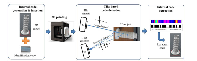
This paper presents an all-in-one encoder/decoder approach for the nondestructive identification of three-dimensional (3D)-printed objects. The proposed method consists of three parts: 3D code insertion, terahertz (THz)-based detection, and code extraction. During code insertion, a relevant one-dimensional (1D) identification code is generated to identify the 3D-printed object. A 3D barcode corresponding to the identification barcode is then generated and inserted into a blank bottom area inside the object's stereolithography (STL) file. For this objective, it is necessary to find an appropriate area of the STL file and to merge the 3D barcode and the model within the STL file. Next the information generated inside the object is extracted by using THz waves that are transmitted and reflected by the output 3D object. Finally, the resulting THz signal from the target object is detected and analyzed to extract the identification information. We implemented and tested the proposed method using a 3D graphic environment and a THz time-domain spectroscopy system. The experimental results indicate that one-dimensional barcodes are useful for identifying 3D-printed objects because they are simple and practical to process. Furthermore, information efficiency can be increased by using an integral fast Fourier transform to identify any code located in areas deeper within the object. As 3D printing is used in various fields, the proposed method is expected to contribute to the acceleration of the distribution of 3D printing empowered by the integration of the internal code insertion and recognition process.

| [1] |
N. Shahrubudin, T. C. Lee, R. Ramlan, An overview on 3D printing technology: Technological, materials, and applications, Procedia Manuf., 35 (2019), 1286–1296. https://doi.org/10.1016/j.promfg.2019.06.089 doi: 10.1016/j.promfg.2019.06.089

|
| [2] |
T. D. Ngo, A. Kashani, G. Imbalzano, K. T. Q. Nguyen, D. Hui, Additive manufacturing (3D printing): A review of materials, methods, applications and challenges, Composites, Part B, 143 (2018), 172–196. https://10.1016/j.compositesb.2018.02.012 doi: 10.1016/j.compositesb.2018.02.012
|
| [3] | M. Nisser, C. C. Liao, Y. Chai, A. Adhikari, S. Hodges, S. Mueller, LaserFactory: A laser cutter-based electromechanical assembly and fabrication platform to make functional devices & robots, in Proceedings of the 2021 CHI Conference on human factors in computing systems, 2021. https://doi.org/10.1145/3411764.3445692 |
| [4] | L. Sun, Y. Yang, Y. Chen, J. Li, D. Luo, H. Liu, et al., ShrinCage: 4D printing accessories that self-adapt, in Proceedings of the 2021 CHI Conference on Human Factors in Computing Systems, 2021. https://doi.org/10.1145/3411764.3445220 |
| [5] | M. Simon, When copyright can kill: How 3D printers are breaking the barriers between "intellectual" property and the physical world, Pace Intell. Prop. Sports & Ent. LF, 3 (2013), 30. https://digitalcommons.pace.edu/pipself/vol3/iss1/4 |
| [6] | M. Holland, C. Nigischer, J. Stjepandić, Copyright protection in additive manufacturing with blockchain approach, in Transdisciplinary Engineering: A Paradigm Shift, 5 (2017), 914–921. https://doi.org/10.3233/978-1-61499-779-5-914 |
| [7] |
T. Rayna, L. Striukova, From rapid prototyping to home fabrication: How 3D printing is changing business model innovation, Technol. Forecasting Social Change, 102 (2016), 214–224. https://doi.org/10.1016/j.techfore.2015.07.023 doi: 10.1016/j.techfore.2015.07.023
|
| [8] |
K. Paraskevoudis, P. Karayannis, E. P. Koumoulos, Real-time 3D printing remote defect detection (stringing) with computer vision and artificial intelligence, Processes, 8 (2020), 1464. https://doi.org/10.3390/pr8111464 doi: 10.3390/pr8111464
|
| [9] |
F. Peng, J. Yang, Z. X. Lin, M. Long, Source identification of 3D printed objects based on inherent equipment distortion, Comput. Secur., 82 (2019), 173–183. https://doi.org/10.1016/j.cose.2018.12.015 doi: 10.1016/j.cose.2018.12.015
|
| [10] | D. Li, A. S. Nair, S. K. Nayar, C. Zheng, AirCode: Unobtrusive physical tags for digital fabrication, in Proceedings of the 30th annual ACM symposium on user interface software and technology, (2017), 449–460. https://doi.org/10.1145/3126594.3126635 |
| [11] | Y. Kubo, K. Eguchi, R. Aoki, 3D-Printed object identification method using inner structure patterns configured by slicer software, in Extended Abstracts of the ACM CHI Conference on Human Factors in Computing Systems, 2020. https://doi.org/10.1145/3334480.3382847 |
| [12] | W. Song, L. Zhang, Y. Tian, S. Fong, J. Liu, A. Gozho, CNN-based 3D object classification using Hough space of LiDAR point clouds, Hum.-centric Comput. Inf. Sci., 10 (2020). https://doi.org/10.1186/s13673-020-00228-8 |
| [13] | Z. Li, A. S. Rathore, C. Song, S. Wei, Y. Wang, W. Xu, PrinTracker: Fingerprinting 3D printers using commodity scanners, in Proceedings of the 2018 ACM sigsac conference on computer and communications security, (2018), 1306–1323. https://doi.org/10.1145/3243734.3243735 |
| [14] |
X. Zhang, L. Bai, Z. Zhang, Y. Li, Multi-scale keypoints feature fusion network for 3D object detection from point clouds, Hum.-centric Comput. Inf. Sci., 12 (2022), 29. https://doi.org/10.22967/HCIS.2022.12.029 doi: 10.22967/HCIS.2022.12.029
|
| [15] |
C. K. Tsung, C. T. Yang, R. Ranjan, Y. L. Chen, J. H. Ou, Performance evaluation of the vSAN application: A case study on the 3D and AI virtual application cloud service, Hum.-centric Comput. Inf. Sci., 11 (2021), 09. https://doi.org/10.22967/HCIS.2021.11.009 doi: 10.22967/HCIS.2021.11.009
|
| [16] | C. Harrison, R. Xiao, S. E. Hudson, Acoustic barcodes: Passive, durable and inexpensive notched identification tags, in Proceedings of the 25th annual ACM symposium on User interface software and technology, (2012), 563–568. https://doi.org/10.1145/2380116.2380187 |
| [17] |
W. L. Chan, J. Deibel, D. M. Mittleman, Imaging with terahertz radiation, Rep. Prog. Phys., 70 (2007), 1325–1379. https://doi.org/10.1088/0034-4885/70/8/R02 doi: 10.1088/0034-4885/70/8/R02
|
| [18] |
A. A. Gowena, C. O'Sullivan, C. P. O'Donnell, Terahertz time domain spectroscopy and imaging: Emerging techniques for food process monitoring and quality control, Trends Food Sci. Technol., 25 (2012), 40–46. https://doi.org/10.1016/j.tifs.2011.12.006 doi: 10.1016/j.tifs.2011.12.006
|
| [19] | C. Shin, Y. Kim, J. Hong, H. Kang, S. H. Hong, Noninvasively detecting internal information of 3D printed objects using terahertz, Int. Inf. Inst. (Tokyo). Inf., 19 (2016), 1575–1580. |
| [20] |
K. D. D. Willis, A. D. Wilson, InfraStructs: Fabricating information inside physical objects for imaging in the terahertz region, ACM Trans. Graphics, 32 (2013), 138. https://doi.org/10.1145/2461912.2461936 doi: 10.1145/2461912.2461936
|
| [21] |
Y. Amarasinghe, H. Guerboukha, Y. Shiri, D. Mittleman, Bar code reader for the THz region, Opt. Express, 29 (2021), 20240–20249. https://doi.org/10.1364/OE.428547 doi: 10.1364/OE.428547
|


Figures(11)

Choonsung Shin, Sung-Hee Hong, Hieyoung Jeong, Hyoseok Yoon, Byoungsoo Koh. All-in-one encoder/decoder approach for non-destructive identification of 3D-printed objects[J]. Mathematical Biosciences and Engineering, 2022, 19(12): 14102-14115. doi: 10.3934/mbe.2022657


 DownLoad: