COVID-19 pandemic control using restrictions and vaccination

Vinicius Piccirillo; Vinicius Piccirillo

doi:10.3934/mbe.2022062

Mathematical Biosciences and Engineering

2022, Volume 19, Issue 2: 1355-1372. doi: 10.3934/mbe.2022062

Previous Article Next Article

Research article

COVID-19 pandemic control using restrictions and vaccination

Vinicius Piccirillo ^,

Department of Mathematics, Federal Technological University of Parana UTFPR, 84016 - 210, Ponta Grossa – PR, Brazil

Received: 28 September 2021 Accepted: 24 November 2021 Published: 03 December 2021

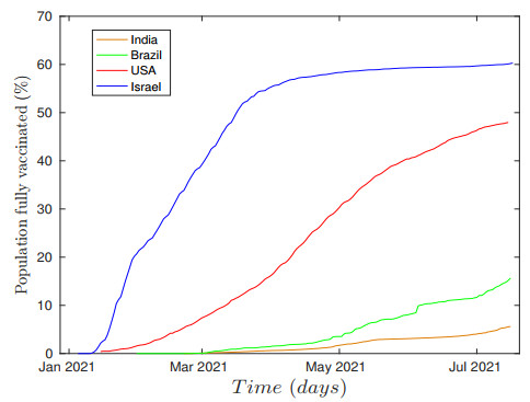
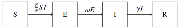
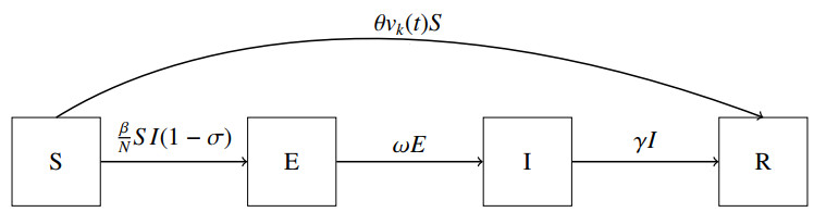
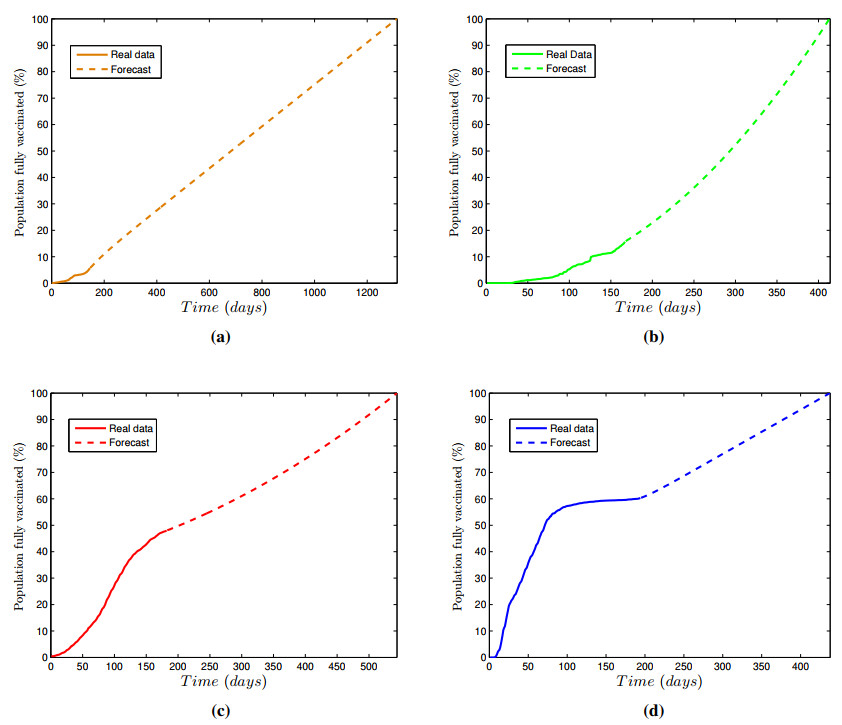
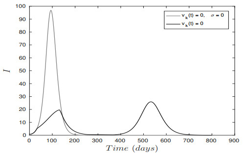
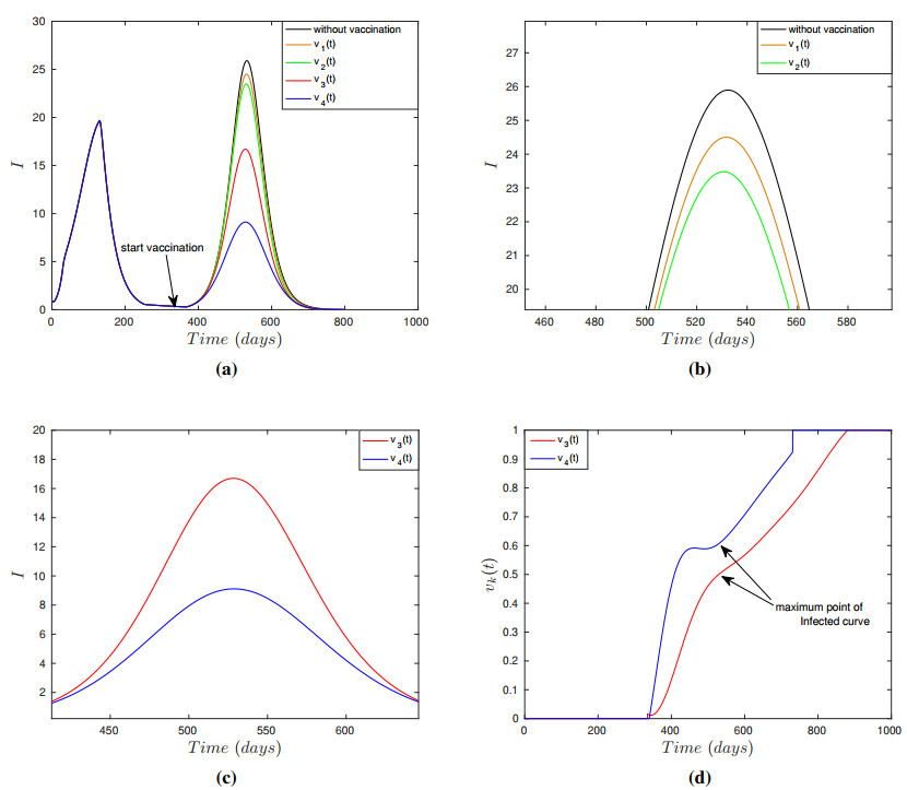
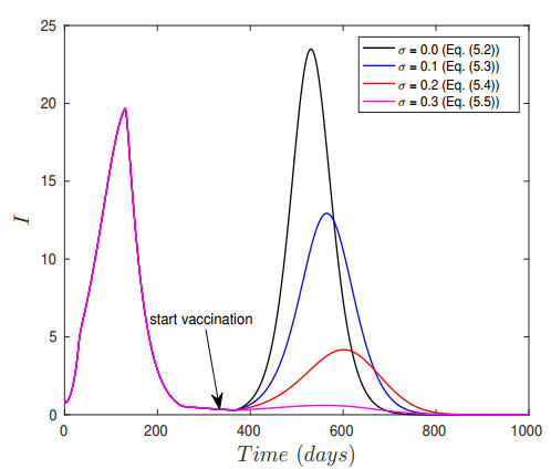
This work deals with the impact of the vaccination in combination with a restriction parameter that represents non-pharmaceutical interventions measures applied to the compartmental SEIR model in order to control the COVID-19 epidemic. This restriction parameter is used as a control parameter, and the univariate autoregressive integrated moving average (ARIMA) is used to forecast the time series of vaccination of all individuals of a specific country. Having in hand the time series of the population fully vaccinated (real data + forecast), the Levenberg–Marquardt algorithm is used to fit an analytic function that models this evolution over time. Here, it is used two time series of real data that refer to a slow vaccination obtained from India and Brazil, and two faster vaccination as observed in Israel and the United States of America. Together with vaccination, two different control approaches are presented in this paper, which enable reduces the infected people successfully: namely, the feedback and nonfeedback control methods. Numerical results predict that vaccination can reduce the peaks of infections and the duration of the pandemic, however, a better result is achieved when the vaccination is combined with any restrictions or prevention policy.
- COVID-19,
- Vaccination,
- Mathematical model,
- Control of infection spread
Citation: Vinicius Piccirillo. COVID-19 pandemic control using restrictions and vaccination[J]. Mathematical Biosciences and Engineering, 2022, 19(2): 1355-1372. doi: 10.3934/mbe.2022062

Related Papers:

Abstract

This work deals with the impact of the vaccination in combination with a restriction parameter that represents non-pharmaceutical interventions measures applied to the compartmental SEIR model in order to control the COVID-19 epidemic. This restriction parameter is used as a control parameter, and the univariate autoregressive integrated moving average (ARIMA) is used to forecast the time series of vaccination of all individuals of a specific country. Having in hand the time series of the population fully vaccinated (real data + forecast), the Levenberg–Marquardt algorithm is used to fit an analytic function that models this evolution over time. Here, it is used two time series of real data that refer to a slow vaccination obtained from India and Brazil, and two faster vaccination as observed in Israel and the United States of America. Together with vaccination, two different control approaches are presented in this paper, which enable reduces the infected people successfully: namely, the feedback and nonfeedback control methods. Numerical results predict that vaccination can reduce the peaks of infections and the duration of the pandemic, however, a better result is achieved when the vaccination is combined with any restrictions or prevention policy.

References

[1]	C. A. Varotsos, V. F. Krapivin, Y. Xue, Diagnostic model for the society safety under COVID-19 pandemic conditions, Saf. Sci., 136 (2021), 105164. doi: 10.1016/j.ssci.2021.105164. doi: 10.1016/j.ssci.2021.105164
[2]	X. Lao, L. Luo, Z. Lei, T. Fang, Y. Chen, Y. Liu, et al., The epidemiological characteristics and effectiveness of countermeasures to contain coronavirus disease 2019 in Ningbo City, Zhejiang Province, China, Sci. Rep., 11 (2021), 1–12. doi: 10.1038/s41598-021-88473-4. doi: 10.1038/s41598-021-88473-4
[3]	S. Jamshidi, M. Baniasad, D. Niyogi, Global to USA county scale analysis of weather, urban density, mobility, homestay, and mask use on COVID-19, Int. J. Environ. Res. Public Health, 17 (2020), 7847. doi: 10.3390/ijerph17217847. doi: 10.3390/ijerph17217847
[4]	A. Huppert, G. Katriel, Mathematical modelling and prediction in infectious disease epidemiology, Clin. Microbiol. Infect., 19 (2013), 999–1005. doi:10.1111/1469-0691.12308. doi: 10.1111/1469-0691.12308
[5]	Coronavirus (COVID-19) in the UK - COVID-19 dataset. https://coronavirus.data.gov.uk/details/about-data, 2021. Accessed on: 2021-11-21.
[6]	M. Baniasad, M. G. Mofrad, B. Bahmanabadi, S. Jamshidi, COVID-19 in Asia: Transmission factors, re-opening policies, and vaccination simulation, Environ. Res., 202 (2021), 111657. doi: 10.1016/j.envres.2021.111657. doi: 10.1016/j.envres.2021.111657
[7]	S. L. de Souza, A. M. Batista, I. L. Caldas, K. C. Iarosz, J. D. Szezech Jr, Dynamics of epidemics: Impact of easing restrictions and control of infection spread, Chaos Solitons Fractals, 142 (2020), 110431. doi: 10.1016/j.chaos.2020.110431. doi: 10.1016/j.chaos.2020.110431
[8]	P. M. Pacheco, M. A. Savi, P. V. Savi, COVID-19 dynamics considering the influence of hospital infrastructure: an investigation into Brazilian scenarios, Nonlinear Dyn., 106 (2021), 1325–1346. doi: 10.1007/s11071-021-06323-4. doi: 10.1007/s11071-021-06323-4
[9]	S. He, Y. Peng, K. Sun, SEIR modeling of the COVID-19 and its dynamics, Nonlinear Dyn., 127 (2020), 1667–1680. doi: 10.1007/s11071-020-05743-y. doi: 10.1007/s11071-020-05743-y
[10]	C. A. Varotsos, V. F. Krapivin, A new model for the spread of COVID-19 and the improvement of safety, Saf. Sci., 132 (2020), 104962. doi: 10.1016/j.ssci.2020.104962. doi: 10.1016/j.ssci.2020.104962
[11]	V. Piccirillo, Nonlinear control of infection spread based on a deterministic SEIR model, Chaos Solitons Fractals, 149 (2021), 111051. doi: 10.1016/j.chaos.2021.111051. doi: 10.1016/j.chaos.2021.111051
[12]	S. Zhai, G. Luo, T. Huang, X. Wang, J. Tao, P. Zhou, Vaccination control of an epidemic model with time delay and its application to COVID-19, Nonlinear Dyn., 106 (2021), 1279–1292. doi: 10.1007/s11071-021-06533-w. doi: 10.1007/s11071-021-06533-w
[13]	K. Prem, L. Yang, W. R. Timothy, J. K. Adam, M. E. Rosalind, D. Nicholas, et al., The effect of control strategies to reduce social mixing on outcomes of the COVID-19 epidemic in Wuhan, China: A modelling study, Lancet Public Health, 55 (2020), 261–270. doi: 10.1016/S2468-2667(20)30073-6. doi: 10.1016/S2468-2667(20)30073-6
[14]	C. N. Ngonghala, E. Iboi, S. Eikenberry, M. Scotch, C. R. MacIntyre, M. H. Bonds, et al., Mathematical assessment of the impact of non-pharmaceutical interventions on curtailing the 2019 novel Coronavirus, Math. Biosci., 325 (2020), 1083. doi: 10.1016/j.mbs.2020.108364. doi: 10.1016/j.mbs.2020.108364
[15]	C. A. Varotsos, V. F. Krapivin, Y. Xue, V. Soldatov, T. Voronova, COVID-19 Pandemic Decision Support System for an Appropriate Population Defense Strategy and Vaccination Effectiveness, Saf. Sci., 142 (2021), 105370. doi: doi.org/10.1016/j.ssci.2021.105370. doi: 10.1016/j.ssci.2021.105370
[16]	R. G. Kavasseri, K. Seetharaman, Day-ahead wind speed forecasting using f-ARIMA models, Renew. Energy, 34 (2009), 1388–1393. doi: 10.1016/j.renene.2008.09.006. doi: 10.1016/j.renene.2008.09.006
[17]	H. B. Hwarng, Insights into neural-network forecasting of time series corresponding to ARMA (p, q) structures, Omega, 29 (2001), 273–289. doi: 10.1016/S0305-0483(01)00022-6. doi: 10.1016/S0305-0483(01)00022-6
[18]	E. Cadenas, W. Rivera, Wind speed forecasting in three different regions of Mexico, using a hybrid ARIMA–ANN model, Renew. Energy, 35 (2010), 2732–2738. doi: 10.1016/j.renene.2010.04.022. doi: 10.1016/j.renene.2010.04.022
[19]	Y. Lai, D. A. Dzombak, Use of the autoregressive integrated moving average (ARIMA) model to forecast near-term regional temperature and precipitation, Weather and Forecasting, 35 (2020), 959–976. doi: 10.1175/WAF-D-19-0158.1. doi: 10.1175/WAF-D-19-0158.1
[20]	R. Katoch, A. Sidhu, An Application of ARIMA Model to Forecast the Dynamics of COVID-19 Epidemic in India, Glob. Bus. Rev. (2021), 0972150920988653. doi: 10.1177/0972150920988653. doi: 10.1177/0972150920988653
[21]	R. C. Das, Forecasting incidences of COVID-19 using Box-Jenkins method for the period July 12-September 11, 2020: A study on highly affected countries, Chaos Solitons Fractals, 140 (2020), 110248. doi: 10.1016/j.chaos.2020.110248. doi: 10.1016/j.chaos.2020.110248
[22]	K. Canfell, H. Chesson, S. L. Kulasingam, J. Berkhof, M. Diaz, J. J. Kim, Modeling preventative strategies against human papillomavirus-related disease in developed countries, Vaccine, 30 (2012), F157–-F167. doi: 10.1016/j.vaccine.2012.06.091. doi: 10.1016/j.vaccine.2012.06.091
[23]	E. Shim, Z. Feng, M. Martcheva, C. Castillo-Chavez, An age-structured epidemic model of rotavirus with vaccination, J. Math. Biol., 53 (2006), 719–-746. doi: 10.1007/s00285-006-0023-0. doi: 10.1007/s00285-006-0023-0
[24]	E. Mathieu, H. Ritchie, E. Ortiz-Ospina, M. Roser, C. Giattino, A global database of COVID-19 vaccinations, Nat. Hum. Behav., 5 (2021), 947–-953. doi: 10.1038/s41562-021-01122-8. doi: 10.1038/s41562-021-01122-8
[25]	G. E. P. Box, G. M. Jenkins, Time Series Analysis. Forecasting and Control, Halden-Day, San Francisco, 1970.
[26]	W. Enders, Applied econometric time series, John Wiley & Sons (2008).
[27]	D. Kwiatkowski, P. C. B. Phillips, P. Schmidt, Y. Shin, Testing the null hypothesis of stationarity against the alternative of a unit root, J. Econom., 54 (1992), 159-–178. doi: 10.1016/0304-4076(92)90104-Y. doi: 10.1016/0304-4076(92)90104-Y
[28]	W. Wang, Stochastic, Nonlinearity and Forecasting of Streamflow. Amsterdan: Deft University Press (2006).
[29]	I. Sandberg, On the mathematical foundations of compartmental analysis in biology, medicine, and ecology, IEEE Trans. Circuits Syst., 25 (1978), 273–279. doi: 10.1109/TCS.1978.1084473. doi: 10.1109/TCS.1978.1084473
[30]	A. J. Kucharski, T. W. Russell, C. Diamond, Y. Liu, J. Edmunds, S. Funk, et al., Early dynamics of transmission and control of COVID-19: a mathematical modelling study, Lancet Infect. Dis., 20 (2020), 553–558. doi: 10.1016/S1473-3099(20)30144-4. doi: 10.1016/S1473-3099(20)30144-4
[31]	J. A. Backer, D. Klinkenberg, J. Wallinga, Incubation period of 2019 novel coronavirus (2019-nCoV) infections among travellers from Wuhan, China, 20–28 January 2020, Euro Surveill, 25 (2020), 2000062. doi: 10.2807/1560-7917.ES.2020.25.5.2000062. doi: 10.2807/1560-7917.ES.2020.25.5.2000062
[32]	R. Woelfel, V. M. Corman, W. Guggemos, M. Seilmaier, C. Wendtner, Clinical presentation and virological assessment of hospitalized cases of coronavirus disease 2019 in a travel-associated transmission cluster, MedRxiv, (2020). doi: 10.1101/2020.03.05.20030502.
[33]	P. Zimmermann, N. Curtis, Factors that influence the immune response to vaccination, Clin. Microbiol. Rev., 32 (2019), e00084-18. doi:10.1128/CMR.00084-18. doi: 10.1128/CMR.00084-18
[34]	J. M. Dan, J. Mateus, Y. Kato, K. M. Hastie, E. D. Yu, C. E. Faliti, et al., Immunological memory to SARS-CoV-2 assessed for up to 8 months after infection, Science, 371 (2021). doi: 10.1126/science.abf4063.
[35]	S. Nusair, Testing the validity of purchasing power parity for asian countries during the current float, J. Econ. Dev., 28 (2003), 129–147.

Reader Comments

Your name:*

Email:*
© 2022 the Author(s), licensee AIMS Press. This is an open access article distributed under the terms of the Creative Commons Attribution License (http://creativecommons.org/licenses/by/4.0)