The role of proactive behavior on COVID-19 infordemic in the Chinese Sina-Microblog: a modeling study

Fulian Yin; Hongyu Pang; Lingyao Zhu; Peiqi Liu; Xueying Shao; Qingyu Liu; Jianhong Wu; Fulian Yin; Hongyu Pang; Lingyao Zhu; Peiqi Liu; Xueying Shao; Qingyu Liu; Jianhong Wu

doi:10.3934/mbe.2021365

Mathematical Biosciences and Engineering

2021, Volume 18, Issue 6: 7389-7401. doi: 10.3934/mbe.2021365

Previous Article Next Article

Research article Special Issues

The role of proactive behavior on COVID-19 infordemic in the Chinese Sina-Microblog: a modeling study

1.
State Key Laboratory of Media Convergence and Communication, Communication University of China, Beijing, 100024, China
2.
College of Information and Communication Engineering, Communication University of China, Beijing 100024, China
3.
The third construction CO.LTD of China construction third engineering bureau Beijing, Beijing 100024, China
4.
Fields-CQAM Laboratory of Mathematics for Public Health, Laboratory for Industrial and Applied Mathematics, York University, Toronto M3J1P3, Canada

Academic Editor: Cameron Nowzari

Received: 30 June 2021 Accepted: 11 August 2021 Published: 30 August 2021

In order to avoid forming an information cocoon, the information propagation of COVID-19 is usually created through the action of "proactive search", an important behavior other than "reactive follow". This behavior has been largely ignored in modeling information dynamics. Here, we propose to fill in this gap by proposing a proactive-reactive susceptible-discussing-immune (PR-SFI) model to describe the patterns of co-propagation on social networks. This model is based on the forwarding quantity and takes into account both proactive search and reactive follow behaviors. The PR-SFI model is parameterized by data fitting using real data of COVID-19 related topics in the Chinese Sina-Microblog, and the model is calibrated and validated using the prediction accuracy of the accumulated forwarding users. Our sensitivity analysis and numerical experiments provide insights about optimal strategies for public health emergency information dissemination.
- Chinese Sina-Microblog,
- active search-reactive follow,
- information propagation model
Citation: Fulian Yin, Hongyu Pang, Lingyao Zhu, Peiqi Liu, Xueying Shao, Qingyu Liu, Jianhong Wu. The role of proactive behavior on COVID-19 infordemic in the Chinese Sina-Microblog: a modeling study[J]. Mathematical Biosciences and Engineering, 2021, 18(6): 7389-7401. doi: 10.3934/mbe.2021365

Related Papers:

Abstract

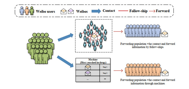
In order to avoid forming an information cocoon, the information propagation of COVID-19 is usually created through the action of "proactive search", an important behavior other than "reactive follow". This behavior has been largely ignored in modeling information dynamics. Here, we propose to fill in this gap by proposing a proactive-reactive susceptible-discussing-immune (PR-SFI) model to describe the patterns of co-propagation on social networks. This model is based on the forwarding quantity and takes into account both proactive search and reactive follow behaviors. The PR-SFI model is parameterized by data fitting using real data of COVID-19 related topics in the Chinese Sina-Microblog, and the model is calibrated and validated using the prediction accuracy of the accumulated forwarding users. Our sensitivity analysis and numerical experiments provide insights about optimal strategies for public health emergency information dissemination.

References

[1]	Q. Gao, F. Abel, G. J. Houben, Y. Yu, A comparative study of users' microblogging behavior on Sina Weibo and Twitter, In Int. Conf. User Model., Adapt., Pers., Springer, Berlin, Heidelberg, (2012), 88–101.
[2]	X. Li, S. Cheng, W. Chen, F. Jiang, Novel User Influence Measurement based on User Interaction in Microblog, 2013 IEEE/ACM Int. Conf. Adv. Soc. Netw. Anal. Min., (2013), 615–619.
[3]	N. Zhang, Y. Chai, Y. Li, H. Sun, Modeling Micro-blog Network Structure based on Combination of Online Communities, in Chin. Contr. Decision Conf., (2013), 3419–3424.
[4]	W. Goffman, V. Newill, Generalization of epidemic theory, Nature, 1964, 204 (1964), 225–228.
[5]	K. Dietz, Epidemics and rumours: A survey, J. R. Stat. Soc. Ser. A (General), 130 (1967), 505–528. doi: 10.2307/2982521
[6]	S. Galam, Modelling rumors: the no plane Pentagon French hoax case, Physica A, 320 (2003), 571–580. doi: 10.1016/S0378-4371(02)01582-0
[7]	S. Abdullah, X. Wu, An epidemic model for news spreading on twitter, 2011 IEEE 23rd Int. Conf. Tools Artif. Intell., IEEE, 2011,163–169.
[8]	B. Zhang, X. Guan, M. J. Khan, Y. Zhou, A time-varying propagation model of hot topic on BBS sites and Blog networks, Inform. Sci., 187 (2012), 15–32. doi: 10.1016/j.ins.2011.09.025
[9]	M. Tanaka, Y. Sakumoto, M. Aida, K. Kawashima, Study on the growth and decline of SNSs by using the infectious recovery SIR model, In 2015 10th Asia-Pacific Symp. Inf. and Telecommun. Technol. (APSITT). IEEE, 2015, 1–3.
[10]	F. Chen, A susceptible-infected epidemic model with voluntary vaccinations, J. Math. Biol., 53 (2006), 253–272. doi: 10.1007/s00285-006-0006-1
[11]	Z. Lu, S. Gao, L. Chen, Analysis of an SI epidemic model with nonlinear transmission and stage structure, Acta Math. Scientia., 23 (2003), 440–446. doi: 10.1016/S0252-9602(17)30486-1
[12]	C. Xia, S. Sun, F. Rao, J. Sun, J. Wang, Z. Chen, SIS model of epidemic spreading on dynamical networks with community, Front. Comput. Sci. China, 3 (2009), 361–365. doi: 10.1007/s11704-009-0057-8
[13]	W. O. Kermack, A. G. McKendrick, Contributions to the mathematical theory of epidemics--I. 1927, Bull. Math. Biol., 53 (1991), 33–55.
[14]	L. Stone, B. Shulgin, Z. Agur, Theoretical examination of the pulse vaccination policy in the SIR epidemic model, Math. Comput. Model., 31 (2000), 207–215. doi: 10.1016/S0895-7177(00)00040-6
[15]	X. Feng, L. Liu, S. Tang, X. Huo, Stability and bifurcation analysis of a two-patch SIS model on
[16]	nosocomial infections, Appl. Math. Lett., 102 (2020), 106097.
[17]	B. Tang, F. Xia, S. Tang, N. L. Bragazzi, Q. Li, X. Sun, et al., The effectiveness of quarantine and isolation determine the trend of the COVID-19 epidemic in the final phase of the current outbreak in China, Int. J. Infect. Dis., 96 (2020), 636–647. doi: 10.1016/j.ijid.2020.05.113
[18]	H. Wang, Y. Li, Z. Feng, L. Feng, ReTweeting analysis and prediction in microblogs: An epidemic inspired approach, China Commun., 10 (2013), 13–24.
[19]	Y. Liu, B. Wang, B. Wu, S. Shang, Y. Zhang, C. Shi, Characterizing super-spreading in microblog: An epidemic-based information propagation model, Physica A, 463 (2016), 202–218. doi: 10.1016/j.physa.2016.07.022
[20]	B. Wang, J. Zhang, H. Guo, Y. Zhang, X. Qiao, Model study of information dissemination in microblog community networks, Discrete Dyn. Nat. Soc., 2016 (2016), 1–11.
[21]	D. Zhao, J. Sun, Y. Tan, J. Wu, Y. Dou, An extended SEIR model considering homepage effect for the information propagation of online social networks, Physica A, 512 (2018), 1019–1031. doi: 10.1016/j.physa.2018.08.006
[22]	Y. Zhang, Y. Feng, R. Yang, Network public opinion propagation model based on the influence of media and interpersonal communication, Int. J. Mod. Phys. B, 33 (2019), 1950393. doi: 10.1142/S0217979219503934
[23]	C. Sang, S. Liao, Modeling and simulation of information dissemination model considering user's awareness behavior in mobile social networks, Physica A, 537 (2020), 122639. doi: 10.1016/j.physa.2019.122639
[24]	A. Kumar, P. Swarnakar, K. Jaiswal, R. Kurele, SMIR model for controlling the spread of information in social networking sites, Physica A, 540 (2020), 122978. doi: 10.1016/j.physa.2019.122978
[25]	X. Chen, N. Wang, Rumor spreading model considering rumor credibility, correlation and crowd classification based on personality, Sci. Rep., 10 (2020), 1–15.
[26]	L. Zhu, W. Liu, Z. Zhang, Delay differential equations modeling of rumor propagation in both homogeneous and heterogeneous networks with a forced silence function, Appl. Math. Comput., 370 (2020), 124925.
[27]	S. H. Choi, H. Seo, M. Yoo, A multi-stage SIR model for rumor spreading, Discrete Contin. Dyn. Syst. Ser. B, 25 (2020), 2351–2372.
[28]	M. Naim, F. Lahmidi, A. Namir, Dynamics of a Delayed Rumor Propagation Model with Consideration of Psychological Factors and Forgetting Mechanism, Appl. Math., 14 (2020), 597–604.
[29]	F. Yin, X. Shao, J. Wu, Nearcasting forwarding behaviors and information propagation in Chinese Sina-Microblog, Math. Biosci. Eng., 16 (2019), 5380–5394. doi: 10.3934/mbe.2019268
[30]	F. Yin, X. Shao, B. Tang, X. Xia, J. Wu, Modeling and analyzing cross-transmission dynamics of related information co-propagation, Sci. Rep., 11 (2021), 1–20. doi: 10.1038/s41598-020-79139-8
[31]	F. Yin, X. Xia, X. Zhang, M. Zhang, J. Lv, J. Wu, Modelling the dynamic emotional information propagation and guiding the public sentiment in the Chinese Sina-microblog, Appl. Math. Comput., 396 (2021), 125884.
[32]	U. L. Abbas, R. M. Anderson, J. W. Mellors, Potential impact of antiretroviral chemoprophylaxis on HIV-1 transmission in resource-limited settings, PloS One, 2 (2007), e875. doi: 10.1371/journal.pone.0000875

Reader Comments

Your name:*

Email:*
© 2021 the Author(s), licensee AIMS Press. This is an open access article distributed under the terms of the Creative Commons Attribution License (http://creativecommons.org/licenses/by/4.0)