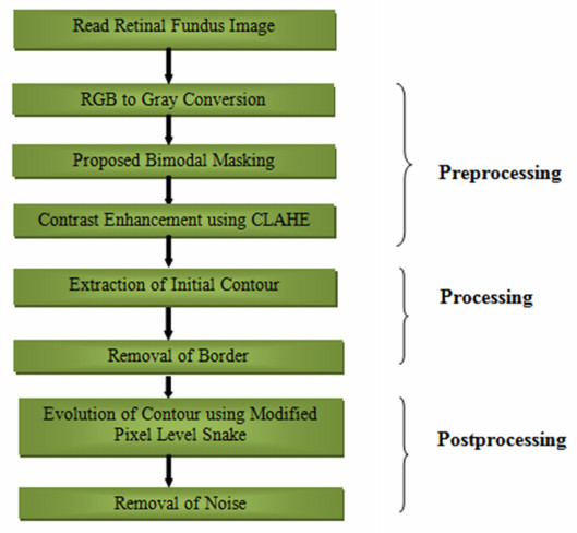
Small changes in retinal blood vessels may produce different pathological disorders which may further cause blindness. Therefore, accurate extraction of vasculature map of retinal fundus image has become a challenging task for analysis of different pathologies. The present study offers an unsupervised method for extraction of vasculature map from retinal fundus images. This paper presents the methodology for evolution of vessels using Modified Pixel Level Snake (MPLS) algorithm based on Black Top-Hat (BTH) transformation. In the proposed method, initially bimodal masking is used for extraction of the mask of the retinal fundus image. Then adaptive segmentation and global thresholding is applied on masked image to find the initial contour image. Finally, MPLS is used for evolution of contour in all four cardinal directions using external, internal and balloon potential. This proposed work is implemented using MATLAB software. DRIVE and STARE databases are used for checking the performance of the system. In the proposed work, various performance metrics such as sensitivity, specificity and accuracy are evaluated. The average sensitivity of 76.96%, average specificity of 98.34% and average accuracy of 96.30% is achieved for DRIVE database. This technique can also segment vessels of pathological images accurately; reaching the average sensitivity of 70.80%, average specificity of 96.40% and average accuracy of 94.41%. The present study provides a simple and accurate method for the detection of vasculature map for normal fundus images as well as pathological images. It can be helpful for the assessment of various retinal vascular attributes like length, diameter, width, tortuosity and branching angle.
Citation: Meenu Garg, Sheifali Gupta, Soumya Ranjan Nayak, Janmenjoy Nayak, Danilo Pelusi. Modified pixel level snake using bottom hat transformation for evolution of retinal vasculature map[J]. Mathematical Biosciences and Engineering, 2021, 18(5): 5737-5757. doi: 10.3934/mbe.2021290
Small changes in retinal blood vessels may produce different pathological disorders which may further cause blindness. Therefore, accurate extraction of vasculature map of retinal fundus image has become a challenging task for analysis of different pathologies. The present study offers an unsupervised method for extraction of vasculature map from retinal fundus images. This paper presents the methodology for evolution of vessels using Modified Pixel Level Snake (MPLS) algorithm based on Black Top-Hat (BTH) transformation. In the proposed method, initially bimodal masking is used for extraction of the mask of the retinal fundus image. Then adaptive segmentation and global thresholding is applied on masked image to find the initial contour image. Finally, MPLS is used for evolution of contour in all four cardinal directions using external, internal and balloon potential. This proposed work is implemented using MATLAB software. DRIVE and STARE databases are used for checking the performance of the system. In the proposed work, various performance metrics such as sensitivity, specificity and accuracy are evaluated. The average sensitivity of 76.96%, average specificity of 98.34% and average accuracy of 96.30% is achieved for DRIVE database. This technique can also segment vessels of pathological images accurately; reaching the average sensitivity of 70.80%, average specificity of 96.40% and average accuracy of 94.41%. The present study provides a simple and accurate method for the detection of vasculature map for normal fundus images as well as pathological images. It can be helpful for the assessment of various retinal vascular attributes like length, diameter, width, tortuosity and branching angle.

| [1] | Z. Yavuz, C. Köse, Blood vessel extraction in color retinal fundus images with enhancement filtering and unsupervised classification, J. Healthcare Eng., 2017 (2017). |
| [2] | J. Lei, X. You, M. Abdel-Mottaleb, Automatic ear landmark localization, segmentation, and pose classification in range images, IEEE Trans. Syst. ManCybern. Syst., 46 (2016), 165-176. |
| [3] | I. Oksuz, J. R. Clough, B. Ruijsink, E. P. Anton, A. Bustin, G. Cruz, et al., Deep learning-based detection and correction of cardiac MR motion artefacts during reconstruction for high-quality segmentation, IEEE Trans. Med. Imaging, 39 (2020), 4001-4010. |
| [4] | M. A. Khan, M. A. Khan, F. Ahmed, M. Mittal, L. M. Goyal, D. J. Hemanth, et al., Gastrointestinal diseases segmentation and classification based on duo-deep architectures, Pattern Recognit. Lett., 131 (2020), 193-204. |
| [5] |
U. T. V. Nguyen, A. Bhuiyan, L. A. F. Park, K. Ramamohanarao, An effective retinal blood vessel segmentation method using multi-scale line detection, Pattern Recognit., 46 (2013), 703-715. doi: 10.1016/j.patcog.2012.08.009

|
| [6] | M. Krause, R. M. Alles, B. Burgeth, J. Weickert, Fast retinal vessel analysis, J. Real Time Image Proc., 11 (2016), 413-422. |
| [7] |
G. Azzopardi, N. Strisciuglio, M. Vento, N. Petkov, Trainable COSFIRE filters for vessel delineation with application to retinal images, Med. Image Anal., 19 (2015), 46-57. doi: 10.1016/j.media.2014.08.002
|
| [8] | S. Roychowdhury, D. D. Koozekanani, K. K. Parhi, Blood vessel segmentation of fundus images by major vessel extraction and subimage classification, IEEE J. Biomed. Heal. Inf., 19 (2015), 1118-1128. |
| [9] |
D. Marín, A. Aquino, M. E. Gegúndez-Arias, J. M. Bravo, A new supervised method for blood vessel segmentation in retinal images by using gray-level and moment invariants-based features, IEEE Trans. Med. Imaging, 30 (2011), 146-158. doi: 10.1109/TMI.2010.2064333
|
| [10] | P. Dai, H. Luo, H. Sheng, Y. Zhao, L. Li, J. Wu, et al., A new approach to segment both main and peripheral retinal vessels based on gray-voting and Gaussian mixture model, PLoS One, 10 (2015), e0127748. |
| [11] | S. Abbasi-Sureshjani, I. Smit-Ockeloen, J. Zhang, B. T. H. Romeny, Biologically-inspired supervised vasculature segmentation in SLO retinal fundus images, Int. Conf. Image Anal. Recognit., 2015 (2015), 325-334. |
| [12] |
J. I. Orlando, E. Prokofyeva, M. B. Blaschko, A discriminatively trained fully connected conditional random field model for blood vessel segmentation in fundus images, IEEE Trans. Biomed. Eng., 64 (2017), 16-27. doi: 10.1109/TBME.2016.2535311
|
| [13] |
N. Strisciuglio, G. Azzopardi, M. Vento, N. Petkov, Supervised vessel delineation in retinal fundus images with the automatic selection of B-COSFIRE filters, Mach. Vis. Appl., 27 (2016), 1137-1149. doi: 10.1007/s00138-016-0781-7
|
| [14] |
E. Ricci, R. Perfetti, Retinal blood vessel segmentation using line operators and support vector classification, IEEE Trans. Med. Imaging, 26 (2007), 1357-1365. doi: 10.1109/TMI.2007.898551
|
| [15] |
M. M. Fraz, A. R. Rudnicka, C. G. Owen, S. A. Barman, Delineation of blood vessels in pediatric retinal images using decision trees-based ensemble classification, Int. J. Comput. Assist. Radiol. Surg., 9 (2014), 795-811. doi: 10.1007/s11548-013-0965-9
|
| [16] | Q. Li, B. Feng, L. Xie, P. Liang, H. Zhang, T. Wang, A cross-modality learning approach for vessel segmentation in retinal images, IEEE Trans. Med. Imaging, 35 (2016), 109-118. |
| [17] | J. S. Kumar, K. Chitra, Segmentation of blood vessels using improved line detection and entropy based thresholding, J. Theor. Appl. Inf. Technol., 63 (2014), 233-239. |
| [18] |
E. Bekkers, R. Duits, T. Berendschot, B. TerHaarRomeny, A multi-orientation analysis approach to retinal vessel tracking, J. Math. Imaging Vis., 49 (2014), 583-610. doi: 10.1007/s10851-013-0488-6
|
| [19] | Y. Chen, Y. Zhang, J. Yang, Q. Cao, G. Yang, J. Chen, et al., Curve-like structure extraction using minimal path propagation with backtracking, IEEE Trans. Image Process., 25 (2016), 988-1003. |
| [20] |
B. Al-Diri, A. Hunter, D. Steel, An active contour model for segmenting and measuring retinal vessels, IEEE Trans.Med. Imaging., 28 (2009), 1488-1497. doi: 10.1109/TMI.2009.2017941
|
| [21] |
Y. Zhao, L. Rada, K. Chen, S. P. Harding, Y. Zheng, Automated vessel segmentation using infinite perimeter active contour model with hybrid region information with application to retinal images, IEEE Trans. Med. Imaging., 34 (2015), 1797-1807. doi: 10.1109/TMI.2015.2409024
|
| [22] |
K. W. Sum, P. Y. S. Cheung, Vessel extraction under non-uniform illumination: A level set approach, IEEE Trans. Biomed. Eng., 55 (2008), 358-360. doi: 10.1109/TBME.2007.896587
|
| [23] | L. Espona, M. J. Carreira, M. G. Penedo, M. Ortega, Retinal vessel tree segmentation using a deformable contour model, Proc. Int. Conf. Pattern Recognit., 2008 (2008), 1-4. |
| [24] | A. Nieto, V. Brea, D. L. Vilariño, R. R. Osorio, Performance analysis of massively parallel embedded hardware architectures for retinal image processing, EURASIP J. Image Video Proc., 2011 (2011), 1-17. |
| [25] | B. Dizdaro, E. Ataer-Cansizoglu, J. Kalpathy-Cramer, K. Keck, M. F. Chiang, D. Erdogmus, Level sets for retinal vasculature segmentation using seeds from ridges and edges from phase maps, IEEE Int. Work. Mach. Learn. Signal Proc., 2012 (2012), 1-6. |
| [26] | Y. Tian, Q. Chen, W. Wang, Y. Peng, Q. Wang, F. Duan, et al., A vessel active contour model for vascular segmentation, Biomed Res. Int., 2014 (2014). |
| [27] | J. Zheng, P. R. Lu, D. Xiang, Y. K. Dai, Z. B. Liu, D. J. Kuai, et al., Retinal image graph-cut segmentation algorithm using multiscale Hessian-enhancement-based nonlocal mean filter, Comput. Math. Methods Med., 2013 (2013). |
| [28] | G. Hassan, N. El-Bendary, A. E. Hassanien, A. Fahmy, S. Abullahm, V. Snasel, Retinal Blood Vessel Segmentation Approach Based on Mathematical Morphology, Procedia Comput. Sci., 2015 (2015), 612-622. |
| [29] |
J. Staal, M. D. Abràmoff, M. Niemeijer, M. A. Viergever, B. Van Ginneken, Ridge-based vessel segmentation in color images of the retina, IEEE Trans. Med. Imaging., 23 (2004), 501-509. doi: 10.1109/TMI.2004.825627
|
| [30] |
J. V. B. Soares, J. J. G. Leandro, R. M. Cesar, H. F. Jelinek, M. J. Cree, Retinal vessel segmentation using the 2-D Gabor wavelet and supervised classification, IEEE Trans. Med. Imaging., 25 (2006), 1214-1222. doi: 10.1109/TMI.2006.879967
|
| [31] |
A. M. Mendonça, A. Campilho, Segmentation of retinal blood vessels by combining the detection of centerlines and morphological reconstruction, IEEE Trans. Med. Imaging., 25 (2006), 1200-1213. doi: 10.1109/TMI.2006.879955
|
| [32] |
M. E. Martinez-Perez, A. D. Hughes, S. A. Thom, A. A. Bharath, K. H. Parker, Segmentation of blood vessels from red-free and fluorescein retinal images, Med. Image Anal., 11 (2007), 47-61. doi: 10.1016/j.media.2006.11.004
|
| [33] |
X. You, Q. Peng, Y. Yuan, Y. M. Cheung, J. Lei, Segmentation of retinal blood vessels using the radial projection and semi-supervised approach, Pattern Recognit., 44 (2011), 2314-2324. doi: 10.1016/j.patcog.2011.01.007
|
| [34] | M. M. Fraz, P. Remagnino, A. Hoppe, B. Uyyanonvara, A. R. Rudnicka, C. G. Owen, et al., An ensemble classification-based approach applied to retinal blood vessel segmentation, IEEE Trans. Biomed. Eng., 59 (2012), 2538-2548. |
| [35] |
C. G. Ravichandran, J. B. Raja, A fast enhancement/thresholding based blood vessel segmentation for retinal image using contrast limited adaptive histogram equalization, J. Med. Imaging Heal. Inf., 4 (2014), 567-575. doi: 10.1166/jmihi.2014.1289
|
| [36] | Y. Q. Zhao, X. H. Wang, X. F. Wang, F. Y. Shih, Retinal vessels segmentation based on level set and region growing, Pattern Recognit., 2014 (2014), 2437-2446. |
| [37] | B. Yin, H. Li, B. Sheng, X. Hou, Y. Chen, W. Wu, et al., Vessel extraction from non-fluorescein fundus images using orientation-aware detector, Med. Image Anal., 26 (2015), 232-242. |
| [38] |
M. Frucci, D. Riccio, G. S. di Baja, L. Serino, Severe: Segmenting vessels in retina images, Pattern Recognit. Lett., 82 (2016), 162-169. doi: 10.1016/j.patrec.2015.07.002
|
| [39] |
J. Zhang, Y. Chen, E. Bekkers, M. Wang, B. Dashtbozorg, B. M. ter H. Romeny, Retinal vessel delineation using a brain-inspired wavelet transform and random forest, Pattern Recognit., 69 (2017), 107-123. doi: 10.1016/j.patcog.2017.04.008
|
| [40] |
C. Alonso-Montes, D. L. Vilariño, P. Dudek, M. G. Penedo, Fast retinal vessel tree extraction: A pixel parallel approach, Int. J. Circuit Theory Appl., 36 (2008), 641-651. doi: 10.1002/cta.512
|
| [41] | R. Perfetti, E. Ricci, D. Casali, G. Costantini, Cellular neural networks with virtual template expansion for retinal vessel segmentation, IEEE Trans. Circuits Syst. Ⅱ Express Briefs., 54 (2007), 141-145. |
| [42] | J. Staal, M. D. Abràmoff, M. Niemeijer, M. A. Viergever, B. van Ginneken, Ridge-based vessel segmentation in color images of the retina, IEEE Trans. Med. Imaging., 23 (2004), 501-509. |
| [43] |
A. Hoover, Locating blood vessels in retinal images by piecewise threshold probing of a matched filter response, IEEE Trans. Med. Imaging., 19 (2000), 203-210. doi: 10.1109/42.845178
|
| [44] |
M. D. Saleh, C. Eswaran, A. Mueen, An automated blood vessel segmentation algorithm using histogram equalization and automatic threshold selection, J. Digit. Imaging., 24 (2011), 564-572. doi: 10.1007/s10278-010-9302-9
|
| [45] |
D. V. S. X. de Silva, W. A. C. Fernando, H. Kodikaraarachchi, S. T. Worrall, A. M. Kondoz, Adaptive sharpening of depth maps for 3D-TV, Electron. Lett., 46 (2010), 1546-1548. doi: 10.1049/el.2010.2320
|
| [46] | K. Ganesan, G. Naik, D. Adapa, A. N. J. Raj, S. N. Alisetti, Z. Zhuang, A supervised blood vessel segmentation technique for digital Fundus images using Zernike Moment based features, PLoS One, 15 (2020), e0229831. |
| [47] | Y. Ma, X. Li, X. Duan, Y. Peng, Y. Zhang, Retinal vessel segmentation by deep residual learning with wide activation, Comput. Intell. Neurosci., 2020 (2020). |
| [48] | M. Li, Z. Ma, C. Liu, G. Zhang, Z. Han, Robust retinal blood vessel segmentation based on reinforcement local descriptions, Biomed Res. Int., 2017 (2017). |


Figures(13) / Tables(3)

Meenu Garg, Sheifali Gupta, Soumya Ranjan Nayak, Janmenjoy Nayak, Danilo Pelusi. Modified pixel level snake using bottom hat transformation for evolution of retinal vasculature map[J]. Mathematical Biosciences and Engineering, 2021, 18(5): 5737-5757. doi: 10.3934/mbe.2021290


 DownLoad: