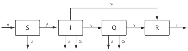
Based on the SIQR model, we consider the influence of time delay from infection to isolation and present a delayed differential equation (DDE) according to the characteristics of the COVID-19 epidemic phenomenon. First, we consider the existence and stability of equilibria in the above delayed SIQR model. Second, we analyze the existence of Hopf bifurcations associated with two equilibria, and we verify that Hopf bifurcations occur as delays crossing some critical values. Then, we derive the normal form for Hopf bifurcation by using the multiple time scales method for determining the stability and direction of bifurcation periodic solutions. Finally, numerical simulations are carried out to verify the analytic results.
Citation: Shishi Wang, Yuting Ding, Hongfan Lu, Silin Gong. Stability and bifurcation analysis of SIQR for the COVID-19 epidemic model with time delay[J]. Mathematical Biosciences and Engineering, 2021, 18(5): 5505-5524. doi: 10.3934/mbe.2021278
[1] | Hongfan Lu, Yuting Ding, Silin Gong, Shishi Wang . Mathematical modeling and dynamic analysis of SIQR model with delay for pandemic COVID-19. Mathematical Biosciences and Engineering, 2021, 18(4): 3197-3214. doi: 10.3934/mbe.2021159 |
[2] | Sarita Bugalia, Jai Prakash Tripathi, Hao Wang . Mathematical modeling of intervention and low medical resource availability with delays: Applications to COVID-19 outbreaks in Spain and Italy. Mathematical Biosciences and Engineering, 2021, 18(5): 5865-5920. doi: 10.3934/mbe.2021295 |
[3] | A. Q. Khan, M. Tasneem, M. B. Almatrafi . Discrete-time COVID-19 epidemic model with bifurcation and control. Mathematical Biosciences and Engineering, 2022, 19(2): 1944-1969. doi: 10.3934/mbe.2022092 |
[4] | Xinyu Liu, Zimeng Lv, Yuting Ding . Mathematical modeling and stability analysis of the time-delayed $ SAIM $ model for COVID-19 vaccination and media coverage. Mathematical Biosciences and Engineering, 2022, 19(6): 6296-6316. doi: 10.3934/mbe.2022294 |
[5] | Yuting Ding, Gaoyang Liu, Yong An . Stability and bifurcation analysis of a tumor-immune system with two delays and diffusion. Mathematical Biosciences and Engineering, 2022, 19(2): 1154-1173. doi: 10.3934/mbe.2022053 |
[6] | Qingwen Hu . A model of regulatory dynamics with threshold-type state-dependent delay. Mathematical Biosciences and Engineering, 2018, 15(4): 863-882. doi: 10.3934/mbe.2018039 |
[7] | Jinhu Xu, Yicang Zhou . Bifurcation analysis of HIV-1 infection model with cell-to-cell transmission and immune response delay. Mathematical Biosciences and Engineering, 2016, 13(2): 343-367. doi: 10.3934/mbe.2015006 |
[8] | Tao Chen, Zhiming Li, Ge Zhang . Analysis of a COVID-19 model with media coverage and limited resources. Mathematical Biosciences and Engineering, 2024, 21(4): 5283-5307. doi: 10.3934/mbe.2024233 |
[9] | Honghua Bin, Daifeng Duan, Junjie Wei . Bifurcation analysis of a reaction-diffusion-advection predator-prey system with delay. Mathematical Biosciences and Engineering, 2023, 20(7): 12194-12210. doi: 10.3934/mbe.2023543 |
[10] | Huan Dai, Yuying Liu, Junjie Wei . Stability analysis and Hopf bifurcation in a diffusive epidemic model with two delays. Mathematical Biosciences and Engineering, 2020, 17(4): 4127-4146. doi: 10.3934/mbe.2020229 |
Based on the SIQR model, we consider the influence of time delay from infection to isolation and present a delayed differential equation (DDE) according to the characteristics of the COVID-19 epidemic phenomenon. First, we consider the existence and stability of equilibria in the above delayed SIQR model. Second, we analyze the existence of Hopf bifurcations associated with two equilibria, and we verify that Hopf bifurcations occur as delays crossing some critical values. Then, we derive the normal form for Hopf bifurcation by using the multiple time scales method for determining the stability and direction of bifurcation periodic solutions. Finally, numerical simulations are carried out to verify the analytic results.
COVID-19 is a respiratory infectious disease and was first reported in Wuhan, China. It is caused by a novel coronavirus named SARS-CoV-2. SARS-COV-2 appeared after severe acute respiratory syndrome coronavirus (SARS) and Middle East respiratory syndrome coronavirus (MERS) [1]. Coronaviruses are enveloped nonsegmented positive-sense RNA viruses and are broadly distributed in mammals, including humans. They can destroy the human respiratory systems and cause severe acute respiratory syndrome [2]. Infected individuals usually cough, have a fever, and have difficulty breathing. Some of them even die of COVID-19. Moreover, there are many ways to spread COVID-19, such as direct transmission, aerosol transmission and contact transmission. This caused COVID-19 to spread rapidly worldwide. As a global infectious disease, COVID-19 has caused more than one million deaths. We attempt to establish a model to analyze the spread of COVID-19 and provide some advice to make COVID-19 controllable.
In recent investigations, many researchers have studied different epidemic models applied to the spread of COVID-19. In ref. [3] and ref. [4], Varotsos et al. established an SPRD model that included people that were susceptible, infected, recovered and dead. The model was based on COVID-19 data and was established to predict COVID-19 spread. We think there is no need to include people who died as a main part of the model because the proportion of people who died is very small. In ref. [5], León et al. developed an SEIARD mathematical model to investigate the COVID-19 outbreak in Mexico. The SEIARD model included infection with symptoms, infection without symptoms (asymptomatic), recovery from symptomatic infection and recovery from asymptomatic infection. If we consider only the infectivity of COVID-19, both infection with symptoms and infection without symptoms (asymptomatic) can infect the suspected cases. There is no need to divide them into infected with symptoms and infected without symptoms (asymptomatic). Both the recovery from symptomatic infection and the recovery from asymptomatic infection have very small possibilities for reinfection. There is no need to divide them into recovered from symptomatic infection and recovered from asymptomatic infection. In ref. [6], an SEIR epidemic model was developed for COVID-19. In ref. [7] and ref. [8], two SIR epidemic models were developed for COVID-19. For COVID-19, many countries have taken quarantine measures, which play an important part in the spread of COVID-19. These authors did not consider the influence of these quarantine measures. The quarantine measures taken by many countries make the proportion of quarantined people large. These quarantine measures can prevent infected individuals from infecting suspected individuals. In addition, exposure to air pollution can damage the heart and lungs and increase vulnerability to more serious coronavirus effects [9]. These quarantine measures can reduce the influence of air pollution. We think it is necessary to consider quarantined people because of the importance of these quarantine measures and the number of quarantined people. We attempt to construct an SIQR epidemic model including quarantined people to describe the spread of COVID-19.
In the spreading process of COVID-19, there is a time delay from infection to isolation. There are some studies about other epidemics with time delays. Liu et al. [10] developed an SEIRU epidemic model with a time delay before an infected person can transmit the infection to another person. They evaluated the effect of the latency period on the dynamics of COVID-19. Xu [11] and Yang et al. [12] also developed epidemic models with time delays before an infected person can transmit the infection to another person. Although this kind of time delay exists, human beings have difficulty changing this kind of time delay. In addition, Wang et al. [13] and Liu et al. [14] made time delays in their models the sojourn times in an infective state. Lu et al. [15] presented an SIQR model with a time delay from infection to recovery. The influence of the time delay from infection to recovery was discussed in detail. According to their conclusions, the smaller the time delay from infection to isolation was, the better COVID-19 was controlled. We decide to focus on the time delay from infection to isolation and discuss the effect of the time delay from infection to isolation on the spread of COVID-19, which is the main difference between our work and the works of others.
Stability and bifurcation have great significance to epidemic models, and some studies have analyzed stability and bifurcation for some epidemic models. In ref. [16], Greenhalgh investigated the stability of some SEIRS epidemiological models with vaccination and temporary immunity. Greenhalgh proposed that there was a threshold parameter R0, and the disease could persist if and only if R0 exceeded one. In addition, disease-free equilibrium always existed and was locally stable if R0<1 and unstable if R0>1. However, for R0>1, the endemic equilibrium was unique and locally asymptotically stable. Based on this conclusion, we think it is necessary for us to calculate the threshold parameter R0 in our model. In ref. [17], Xie et al. investigated the global stability of endemic equilibrium of an SIS epidemic model in complex networks. They proved that the endemic equilibrium was globally asymptotically stable by using a combination of the Lyapunov function method and a monotone iterative technique. However, the Hopf bifurcation analysis was not mentioned in this paper. In refs. [18,19], two SIS models were proposed. In ref. [20], an SIQRS model was proposed. The stability of the models was analyzed, but bifurcation analysis was not mentioned. In refs. [21,22,23,24], the stability and bifurcation of some SIR models were analyzed by different authors. In refs. [25,26,27,28], different SIR models were developed. The stability and bifurcation of them were analyzed. In ref. [29], an SIR epidemic model with time delay was proposed. In ref. [30], an SIR model with information-dependent vaccination was proposed. We compare the methods they used to analyze the stability and bifurcation of these SIR models. Then, we use the multiple time scales method, which was also used in ref. [21]. The multiple time scales method is systematic. It is a standard method for calculating the normal form of Hopf bifurcation. It can be directly applied to the original nonlinear dynamical system, which is described by ordinary differential equations and delayed differential equations, without application of the center manifold theory [31].
It is obvious that the isolation measures taken by many countries play an important role in controlling the spread of COVID-19. The time delay also has a considerable influence on the spread. Thus, we attempt to develop one mathematical model with a time delay to investigate the spread of COVID-19 and analyze the stability of this model. In some studies such as refs. [3,4,5], the authors forecasted how the epidemic situation changed with detailed data. However, we decide to focus on the stability of equilibria in our model, calculate the critical time delay from infection to isolation and analyze the dynamical property of our model to discuss the tendency of the spread of COVID-19.
The main objective of this paper includes constructing the DDE model for COVID-19 and analyzing the stability of the model, the existence of Hopf bifurcation and the stability of the bifurcating periodic solution. The rest of the paper is organized as follows. In Section 2, we construct the DDE model according to the characteristics of the spread of COVID-19. In Section 3, we analyze the existence and stability of the equilibria and the existence of Hopf bifurcation associated with the COVID-19 model with a time delay. We calculate the critical time delay from infection to isolation and analyze the dynamic properties of our model. In Section 4, we derive the normal form of the Hopf bifurcation for the above model and analyze the stability of the bifurcating periodic solution. In Section 5, we present the results of simulations to verify the correctness of our analysis. Finally, the conclusion is drawn in Section 6.
Suspected individuals can be infected with COVID-19 by infected individuals. After individuals are infected with COVID-19, some of them will be quarantined, and some of them will die of COVID-19. The quarantined individuals will not infect others. For COVID-19, we ignore the effect of reinfection because the probability of reinfection is very small. In addition, we ignore the probability of transforming the suspected individuals into recovered individuals directly since the probability is also small. We divide people into four kinds (suspected, infected, quarantined and recovered) based on their infectivity. The specific conversion between the four kinds of people is given in Figure 1.
The variables and parameters in Figure 1 are given in Table 1.
Symbol | Definition |
S | The number of suspected people |
I | The number of infected people |
Q | The number of quarantined people |
R | The number of recovered people |
Λ | The population growth |
μ | The natural mortality |
α1 | The rate of COVID-19 death of infected people |
α2 | The rate of COVID-19 death of quarantined people |
β | The transmission rate from S to I |
ε | The transmission rate from I to Q |
γ1 | The transmission rate from I to R |
γ2 | The transmission rate from Q to R |
For COVID-19, there is a latent period after the suspected individuals are infected. In the latent period, the infected individuals have no symptoms. However, these asymptomatic infected individuals can also infect suspected individuals. If we consider only their infectivity, there is little difference between asymptomatic infected individuals and symptomatic infected individuals. Thus, both of them can be divided into infected. Additionally, some suspected individuals may be quarantined, and they will not be infected. This means that the number of suspected persons who can be infected will decrease. Considering the influence of the suspected individuals who are quarantined, we can reduce the transmission rate from S to I, and there is no need to include the suspected individuals who are quarantined in the model.
Based on Figure 1, we construct the DDE model (2.1):
{S′(t)=Λ−μS(t)−βS(t)I(t),I′(t)=βS(t)I(t)−εI(t−τ)−μI(t)−α1I(t)−γ1I(t),Q′(t)=εI(t−τ)−γ2Q(t)−α2Q(t)−μQ(t),R′(t)=γ1I(t)+γ2Q(t)−μR(t), | (2.1) |
where the definitions of parameters and variables are presented in Figure 1 and Table 1, and τ>0 denotes the time delay from infection to isolation.
The initial condition of system (2.1) is ϕS(θ)≥0,ϕI(θ)≥0,ϕQ(θ)≥0,ϕR(θ)≥0, where Φ=(ϕS(θ),ϕI(θ),ϕQ(θ),ϕR(θ))∈C([−τ,0],R4+0) for θ∈[−τ,0], and C([−τ,0],R4+0) is the Banach space of continuous functions mapping interval [−τ,0] into R4+0. For the system (2.1), R4+0={(S,I,Q,R)|S≥0,I≥0,Q≥0,R≥0}.
According to the initial condition of system (2.1), we present a theorem addressing the nonnegativity and the boundedness of the solution to system(2.1).
Theorem 2.1. If S(0)≥0,I(0)≥0,Q(0)≥0,R(0)≥0, the solution S∗(t), I∗(t), Q∗(t), R∗(t) to system (2.1) with τ=0 is nonnegative and bounded when t>0.
Proof. First, we prove S∗(t)≥0 when t≥0 under the initial condition of system (2.1).
We assume that S∗(t) is not always nonnegative for t≥0 and make t1 the first time that S∗(t1)=0, S′(t1)<0. According to the first equation of system (2.1), we can obtain S′(t1)=Λ>0. The two conclusions we obtain are contradictory.
Therefore, S∗(t)≥0 when t>0. In the same way, I∗(t)≥0, Q∗(t)≥0, R∗(t)≥0 when t>0. The solution to system (2.1) is positive when t>0.
Then, let N(t)=S(t)+I(t)+Q(t)+R(t), and N(t) represent the total number of people at time t.
Add four equations of Eq. (2.1), and we obtain N′(t)=Λ−μ(S(t)+I(t)+Q(t)+R(t)). Then, we can obtain limt→∞supN(t)=Λμ. Thus, the solution S∗(t), I∗(t), Q∗(t), R∗(t) to system (2.1) is bounded when t>0.
Remark 1: We prove if S(0)≥0,I(0)≥0,Q(0)≥0,R(0)≥0, the solution S∗(t), I∗(t), Q∗(t), R∗(t) to system (2.1) with τ=0 is positive. It is not easy for us to prove that the solution to system (2.1) is positive when τ>0. However, according to our numerical simulation, we can find that when system (2.1) is stable, the solution to system (2.1) is always positive, which is not contradictory to the positivity of the solution to system (2.1).
Next, we consider the dynamic phenomena of system (2.1).
In this section, the system (2.1) is considered, and we first determine the equilibria of the above system. Obviously, the system (2.1) has two equilibria:
E1=(S∗1,I∗1,Q∗1,R∗1),E2=(S∗2,I∗2,Q∗2,R∗2), | (3.1) |
with
S∗1=Λμ,I∗1=0,Q∗1=0,R∗1=0,S∗2=ε+μ+α1+γ1β,I∗2=Λε+μ+α1+γ1−μβ,Q∗2=εα2+γ2+μ(Λε+μ+α1+γ1−μβ),R∗2=1μ(γ1+εγ2α2+γ2+μ)(Λε+μ+α1+γ1−μβ). | (3.2) |
Transferring the equilibria Ek(k=1,2) to the origin, we make w=S+S∗k, x=I+I∗k, y=Q+Q∗k, z=R+R∗k. We can obtain S=w−S∗k, I=x−I∗k, Q=y−Q∗k and R=z−R∗k. Substituting these equations into the model (2.1), we use S, I, Q and R to represent w, x, y and z. We obtain the following model:
{S′(t)=−μS(t)−βS(t)I(t)−βS∗kI(t)−βS(t)I∗k,I′(t)=βS(t)I(t)+βS∗kI(t)+βS(t)I∗k−εI(t−τ)−μI(t)−α1I(t)−γ1I(t),Q′(t)=εI(t−τ)−γ2Q(t)−α2Q(t)−μQ(t),R′(t)=γ1I(t)+γ2Q(t)−μR(t),k=1,2. | (3.3) |
In this subsection, we first demonstrate the stability of the equilibrium E1=(S∗1,I∗1,Q∗1,R∗1)=(Λμ,0,0,0). We obtain the characteristics equation of the linearized system of Eq. (3.3) at the equilibrium E1 as follows:
(λ+μ)2(λ+μ+α2+γ2)(λ+μ+α1+γ1−βS∗1+εe−λτ)=0. | (3.4) |
When τ=0, Eq. (3.4) becomes:
(λ+μ)2(λ+μ+α2+γ2)(λ+μ+α1+γ1−βS∗1+ε)=0. | (3.5) |
We show the following assumption:
(H1) βS∗1−(ε+μ+α1+γ1)<0.
Under (H1), the four roots of Eq. (3.5) have negative real parts due to μ>0,α1>0,γ1>0, and the equilibrium E1 is locally asymptotically stable when τ=0.
Similarly, for the stability of the other equilibrium E2=(S∗2,I∗2,Q∗2,R∗2), we obtain the characteristic equation of the linearized system of Eq. (3.3) at the equilibrium E2 as follows:
(λ+μ)(λ+μ+α2+γ2)[(λ−ε+εe−λτ)(λ+μ+βI∗2)+β2S∗2I∗2]=0. | (3.6) |
When τ=0, Eq. (3.6) becomes:
(λ+μ)(λ+μ+α2+γ2)[λ2+λ(μ+βI∗2)+β2S∗2I∗2]=0. | (3.7) |
If (H1) is not satisfied, the four roots of Eq. (3.7) have negative real parts due to μ>0,α2>0,γ2>0, and the equilibrium E2 of system (2.1) is locally asymptotically stable when τ=0.
We can find that E1 is the disease-free equilibrium, and E2 is the endemic equilibrium. We calculate the basic reproduction number R0, which is the number of suspected individuals who are infected by the same infectious individual and can estimate the infectiousness of an infectious disease. According to the system (2.1), we can obtain the new infections matrix F and the transition matrix V.
F=[0βS(t)I(t)00],V=[−Λ+μS(t)+βS(t)I(t)εI(t)+μI(t)+α1I(t)+γ1I(t)−εI(t)+γ2Q(t)+α2Q(t)+μQ(t)−γ1I(t)−γ2Q(t)+μR(t)]. |
Then, we make F0 represent the derivative of F at E1 and V0 represent the derivative of V at E1:
F0=[00000βS∗10000000000],V0=[μβS∗1000ε+μ+α1+γ1000−εγ2+α2+μ00−γ1−γ2 μ]. |
The inverse of V0 is:
V−10=[1μ−βS∗1μ(ε+μ+α1+γ1)0001ε+μ+α1+γ1000ε(ε+μ+α1+γ1)(γ2+α2+μ)1γ2+α2+μ001μ[γ1ε+μ+α1+γ1+εγ2(ε+μ+α1+γ1)(γ2+α2+μ)]γ2μ(γ2+α2+μ)1μ.]. |
And we can obtain:
F0V−10=[00000βS∗1ε+μ+α1+γ10000000000]. |
The maximum eigenvalue of F0V−10 is R0:
R0=ρ(F0V−10)=βS∗1ε+μ+α1+γ1. |
We compare R0 with (H1), and we find that if R0<1, the inequality of (H1) exists constantly, and if R0>1, (H1) is not satisfied. This represents if R0<1, the disease-free equilibrium E1 is locally asymptotically stable when τ=0 and if R0>1, the endemic equilibrium E2 is locally asymptotically stable when τ=0.
For equilibrium E1, when τ>0, let λ=iω0(ω0>0) be a root of the following equation:
λ+μ+α1+γ1−βS∗1+εe−λτ=0. | (3.8) |
Substituting λ=iω0 into Eq. (3.8) and separating the real and imaginary parts, we have
{ω0=εsin(ω0τ),βS∗1−(μ+α1+γ1)=εcos(ω0τ). | (3.9) |
Thus, we obtain:
{Q1≜sin(ω0τ)=ω0ε,P1≜cos(ω0τ)=βS∗1−(μ+α1+γ1)ε. | (3.10) |
Adding the square of two equations (3.9), we can obtain
ω20=ε2−[βS∗1−(μ+α1+γ1)]2. | (3.11) |
Thus, ω0=√ε2−[βS∗1−(μ+α1+γ1)]2 when ε2−[βS∗1−(μ+α1+γ1)]2≥0, and substituting it into Eq. (3.10). Since ω0>0 and ε≥0, we can obtain Q1>0 and obtain:
τ(j)1=1ω0[arccos(P1)+2jπ],Q1≥0, | (3.12) |
where Q1,P1 are given in Eq. (3.10), j=0,1,2⋯.
Let λ(τ)=α(τ)+iω(τ) be the root of Eq. (3.8) satisfying α(τ(j)1)=0,ω(τ(j)1)=ω0,j=0,1,2⋯. Then, we have the transversality conditions
Re(dλdτ)−1|λ=iω0,τ=τ(j)1=1ε2>0,j=0,1,2⋯. |
Thus, the system (2.1) undergoes a Hopf bifurcation at equilibrium E1 of system (2.1) when τ=τ(j)1,j=0,1,2,⋯.
For the other equilibrium E2, when τ>0, let λ=iω(ω>0) be the root of the following equation:
(λ−ε+εe−λτ)(λ+μ+βI∗2)+β2S∗2I∗2=0. | (3.13) |
Substituting it into the equation and separating the real and imaginary parts, we have
{ω2+με+εβI∗2−β2S∗2I∗2=(ωε)sin(ωτ)+(με+βεI∗2)cos(ωτ),μω−εω+βωI∗2=(−ωε)cos(ωτ)+(με+βεI∗2)sin(ωτ). | (3.14) |
Equation (3.14) can be presented as:
{Q2≜sin(ωτ)=(ω2+ε(βI∗2+μ)−β2S∗2I∗2)ω−(ε−(βI∗2+μ))(βI∗2+μ)ωε[ω2+(βI∗2+μ)2],P2≜cos(ωτ)=(ω2+ε(βI∗2+μ)−β2S∗2I∗2)(βI∗2+μ)+(ε−(βI∗2+μ))ω2ε[ω2+(βI∗2+μ)2]. | (3.15) |
Adding the square of two equations Eq. (3.14), let z=ω2, and
h(z)=z2+c1z+c0=0, | (3.16) |
where c1=(βI∗2+μ)2−2β2S∗2I∗2,c0=(β2S∗2I∗2)2−2β2S∗2I∗2(βI∗2+μ)ε.
Therefore, we have the following assumption:
(H2) c21−4c0>0,c1<0,c0>0.
(H3) c0<0.
If (H2) holds, then Eq. (3.16) has two positive roots, z1 and z2 (z1<z2). If (H3) holds, then Eq. (3.16) has only one positive root z3. Without loss of generality, substituting ωk=√zk(k=1,2,3) into Eq. (3.15), we obtain:
τ(j)2,k={1ωk[arccos(P2,k)+2jπ],Q2,k≥0,1ωk[2π−arccos(P2,k)+2jπ],Q2,k<0,j=0,1,2⋯, | (3.17) |
where Q2,P2 are given in Eq. (3.15) and Q2,k=Q2|ω=ωk,τ=τ(j)2,k,P2,k=P2|ω=ωk,τ=τ(j)2,k,k=1,2,3.
Note that since Q1=ω0ε is always nonnegative, we can obtain τ(j)1 directly. However, whether Q2 is positive depends on the parameters of Eq. (3.15), and we need to obtain τ(j)2,k, (j=1,2,3) according to the value of Q2.
Furthermore, let λ(τ)=α(τ)+iωk(τ) be the root of Eq. (3.17) satisfying α(τ(j)2,k)=0, ω(τ(j)2,k)=ωk(k=1,2,3;j=0,1,2…).
If (H2) or (H3) holds and zk=ω2k(k=1,2,3), then we can deduce Re(dτdλ)|τ=τ(j)2,k:
Re(dτdλ)|τ=τ(j)2,k=ωk2[(βI∗2+μ)2−2β2S∗2I∗2]ε2[ωk2+(βI∗2+μ)2]=ωk2h′(zk)ε2[ωk2+(βI∗2+μ)2]≠0,k=1,2,3. |
There is a Hopf bifurcation at equilibrium E2 of system (2.1) when τ=τ(j)2,k,j=0,1,2⋯.
Then, we present a stability theorem of system (2.1)'s equilibria E1, E2 and the existence of Hopf bifurcation.
Theorem 3.1. We consider the model (2.1):
(1) If (H1) holds, the equilibrium E1 of the model (2.2) undergoes a Hopf bifurcation when τ=τ(j)1,j=0,1,2⋯, and we obtain the following. When τ∈[0,τ(0)1), the equilibrium E1 is locally asymptotically stable. When τ∈[τ(0)1,+∞), the equilibrium E1 is locally asymptotically unstable.
(2) Under the condition that (H1) is not satisfied, and if (H2) or (H3) holds, the equilibrium E2 of the model (2.1) undergoes a Hopf bifurcation when τ=τ(j)2,k(k=1,2,3), and we obtain the following.
(a) If (H2) holds, h(z) has two positive roots, z1 and z2; then we assume z1<z2, and we obtain h′(z1)<0,h′(z2)>0. Then, ∃m∈N, which can make 0<τ(0)2,2<τ(0)2,1<τ(1)2,2<τ(1)2,1<⋯<τ(m−1)2,1<τ(m)2,2<τ(m+1)2,2. When τ∈[0,τ(0)2,2)∪m⋃l=1(τ(l−1)2,1,τ(l)2,2), the equilibrium of the model is locally asymptotically stable. When τ∈m−1⋃l=0(τ(l)2,2,τ(l)2,1)∪(τ(m)2,2,+∞), the equilibrium is locally asymptotically unstable.
(b) If (H3) holds, h(z) has only one positive root z3, when τ∈[0,τ(0)2,3), the equilibrium E2 is locally asymptotically stable. When τ∈(τ(0)2,3,+∞), the equilibrium E2 is unstable.
Without loss of generality, we denote the critical value τ=τ∗ when the characteristic Eq. (3.4) and Eq. (3.6) have eigenvalue λ=iω∗k,k=1,2, at which system (2.1) undergoes a Hopf bifurcation at equilibrium Ek=(S∗k,I∗k,Q∗k,R∗k),k=1,2.
First, we transform the equilibrium to the origin; then, we use the multiple time scales method, and system (2.1) can be written as
˙X(t)=AX(t)+BX(t−τ)+F(X(t),X(t−τ)), | (4.1) |
where X(t)=(^Sk(t),^Ik(t),^Qk(t),^Rk(t))T, X(t−τ)=(^Sk(t−τ),^Ik(t−τ),^Qk(t−τ),^Rk(t−τ))T,
A=[−μ−βI∗k−βS∗k00βI∗kβS∗k−(μ+α1+γ1)0000−(γ2+α2+μ)00γ1γ2−μ],B=[00000−ε000ε000000],F(X(t),X(t−τ))=[FSFIFQFR]=[Λ−μS∗k−βSkIk−βS∗kI∗kβSkIk+βS∗kI∗k−(ε+μ+α1+γ1)I∗kεI∗k−(μ+α2+γ2)Q∗kγ1I∗k+γ2Q∗k−μR∗k]. |
We make ˜˙X(t)=AX(t)+BX(t−τ) the linear system of system (4.1). We assume that hk(k=1,2) is the eigenvector of the eigenvalue λ=iω∗k(k=1,2) of the linear system and that h∗k is the eigenvector of the eigenvalue λ=−iω∗k of the linear system. We make ˜I the unit matrix, and hk satisfies (λ˜I−A−Be−λτ)hk=0, where λ=iω∗k, and h∗k satisfies (λ˜I−A−Be−λτ)Thk∗=0, where λ=−iω∗k. Additionally, ⟨h∗k,hk⟩=¯h∗kThk=1, and we can obtain
hk=(hk1,hk2,hk3,hk4)T=(−βS∗kλ+μ+βI∗k,1,εe−λτλ+μ+α2+γ2,γ1λ+μ+γ2εe−λτ(λ+μ)(λ+μ+α2+γ2))T,hk∗=(h∗k1,h∗k2,h∗k3,h∗k4)T=dk(βI∗kλ+μ+βI∗k,1,0,0)T, | (4.2) |
where dk=(−β2S∗kI∗k(μ+βI∗k)2+ω∗k2+1)−1,k=1,2.
We use the multiple time scale method to deduce the normal form of the Hopf bifurcation and assume the solution to Eq. (4.1) is
X(t)=X(T0,T1,T2,⋯)=∞∑k=1ϵkXk(T0,T1,T2,⋯), | (4.3) |
where X(T0,T1,T2,⋯)=[S(T0,T1,T2,⋯),I(T0,T1,T2,⋯),Q(T0,T1,T2,⋯),R(T0,T1,T2,⋯)]T, Xk(T0,T1,T2,⋯)=[Sk(T0,T1,T2,⋯),Ik(T0,T1,T2,⋯),Qk(T0,T1,T2,⋯),Rk(T0,T1,T2,⋯)]T, k=1,2, Ti=ϵit,i=0,1,2,⋯ and Ti is the scaling transform in the time direction.
The derivative with respect to t is
ddt=∂∂T0+ϵ∂∂T1+ϵ2∂∂T2+⋯=D0+ϵD1+ϵ2D2+⋯, |
where Di=∂∂Ti,i=0,1,2,⋯.
Note that Xj=(Sj,Ij,Qj,Rj)T=Xj(T0,T1,T2,⋯),Xj,τc=(Sj,τc,Ij,τc,Qj,τc,Rj,τc)T=Xj(T0−τc,T1,T2,⋯),j=1,2,⋯.
Then, we can obtain
⋅X(t)=ϵD0X1+ϵ2D1X1+ϵ3D2X1+ϵ2D0X2+ϵ3D1X2+ϵ3D0X3+⋯. | (4.4) |
We consider that τ is the bifurcation parameter, and we set τ=τc+ϵτε, where τc=τ(j)k(k=1,2) is the critical value of the Hopf bifurcation, τε is the perturbation parameter, and ϵ is the dimensionless parameter.
Using Taylor series expansion of X(t−τ), we obtain that
X(t−τ)=ϵX1,τc+ϵ2X2,τc+ϵ3X3,τc−ϵ2τεD0X1,τc−ϵ3τεD0X2,τc−ϵ2τcD1X1,τc−ϵ3τεD1X1,τc−ϵ3τcD2X1,τc−ϵ3τcD1X2,τc+⋯, | (4.5) |
where Xj,τc=Xj(T0−τc,T1,T2,⋯),j=1,2,⋯.
Then, substituting the solution with the multiple scales Eqs. (4.3)-(4.5) into Eq. (4.1) and balancing the coefficients of ϵn(n=1,2,3), we obtain a set-ordered linear differential equation:
{D0Sk1+(μ+βI∗k)Sk1+βS∗kIk1=0,D0Ik1−βI∗kSk1+(μ+α1+γ1)Ik1−βS∗kIk1+εIk1,τc=0,D0Qk1+(μ+α2+γ2)Qk1−εQk1,τc=0,D0Rk1−γ1Ik1−γ2Qk1+μRk1=0,k=1,2. | (4.6) |
Since ±iω∗k(k=1,2) are the eigenvalues of the characteristic Eq. (4.1), the solution to Eq. (4.6) can be expressed in the form of Eq. (4.7):
X1(T1,T2,T3,⋯)=G1(T1,T2,T3,⋯)eiω∗kT0hk+ˉG1(T1,T2,T3,⋯)e−iω∗kT0ˉhk,k=1,2. | (4.7) |
where G1 and ˉG1 represent the coordinates on the center manifold, and the linear part of the center manifold can be presented as equation (4.7).
Next, for the ϵ2-order terms, we can obtain the following equations:
{D0Sk2+(μ+βI∗k)Sk2+βS∗kIk2=−D1Sk1−βSk1Ik1,D0Ik2−βI∗kSk2+(μ+α1+γ1)Ik2−βS∗kIk2+εIk2,τc=ετεD0Ik1,τc+ετcD1Ik1,τc−D1Ik1+βSk1Ik1,D0Qk2+(μ+α2+γ2)Qk2−εQk2,τc=−ετεD0Qk1,τc−ετcD1Qk1,τc−D1Qk1,D0Rk2−γ1Ik2−γ2Qk2+μRk2=−D1Rk1,k=1,2. | (4.8) |
We substitute Eq. (4.7) into the right expression of Eq. (4.8), and the coefficients before eiω∗kT0 are denoted by the vector m1. According to the solvability condition ⟨h∗k,m1⟩=0, we can solve ∂G∂T1 as follows:
∂G1∂T1=MkτεG1, | (4.9) |
where Mk=εe−iω∗kτc[βI∗k(iω∗k+μ+βI∗k)(μ+βI∗k)2+ω∗k2βS∗kiω∗k+μ+βI∗k+1−ετce−iω∗kτc]−1,k=1,2.
We assume:
Sk2=fk1eiω∗kT0G1+ˉfk1e−iω∗kT0ˉG1+gk1e2iω∗kT0G12+ˉgk1e−2iω∗kT0ˉG12+lk1G1ˉG1,Ik2=fk2eiω∗kT0G1+ˉfk2e−iω∗kT0ˉG1+gk2e2iω∗kT0G12+ˉgk2e−2iω∗kT0ˉG12+lk2G1ˉG1,Qk2=fk3eiω∗kT0G1+ˉfk3e−iω∗kT0ˉG1+gk3e2iω∗kT0G12+ˉgk3e−2iω∗kT0ˉG12+lk3G1ˉG1,Rk2=fk2eiω∗kT0G1+ˉfk4e−iω∗kT0ˉG1+gk4e2iω∗kT0G12+ˉgk4e−2iω∗kT0ˉG12+lk4G1ˉG1. | (4.10) |
Substituting Eq. (4.10) into Eq. (4.8), we obtain:
fk1=U−1τε(iω∗k+μ+α2+γ2−εe−iω∗kτc)[(−Mkhk1)(iω∗k+μ+α1+γ1−βS∗k+εe−iω∗kτc)−βS∗k(iω∗kεe−iω∗kτchk2+ετcMkhk2−Mkhk2)](iω∗k+μ),fk2=U−1τε(iω∗k+μ+α2+γ2−εe−iω∗kτc)[(iω∗k+μ+βI∗k)(iω∗kεe−iω∗kτchk2+ετcMkhk2−Mkhk2)+βI∗k(−Mkhk1)](iω∗k+μ),fk3=τε(iω∗k+μ)[(iω∗k+μ+βI∗k)(iω∗k+μ+α1+γ1−βS∗k+εe−iω∗kτc)(iω∗k+μ+α2−εe−iω∗kτc+γ2)+β2S∗kI∗k(iω∗k+μ+α2+γ2−εe−iω∗kτc)]U−1,fk4=τε{(iω∗k+μ+βI∗k)[(−Mkhk4)(iω∗k+μ+α1+γ1−βS∗k+εe−iω∗kτc)(iω∗k+μ−εe−iω∗kτc+α2+γ2)+γ1(iω∗kεe−iω∗kτchk2+ετcMkhk2−Mkhk2)(iω∗k+μ+α2+γ2−εe−iω∗kτc)+γ2(iω∗k+μ+α1+γ1−βS∗k+εe−iω∗kτc)(−Mkhk3−ετεMke−iω∗kτchk3−iω∗kεe−iω∗kτchk3)]+βI∗k[βS∗k(iω∗k+μ+α2+γ2−εe−iω∗kτc)(−Mkhk4)+γ1(iω∗kεe−iω∗kτchk2+ετcMkhk2−Mkhk2)(iω∗k+μ+α2+γ2−εe−iω∗kτc)+γ2βS∗k(−Mkhk3−iω∗kεMke−iω∗kτchk3−εe−iω∗kτchk3)]}U−1,gk1=(2iω∗k+μ)(2iω∗k+μ+α2+γ2−εe−2iω∗kτc)[(−βhk1hk2)(2iω∗k+μ+α1+γ1+εe−2iω∗kτc−βS∗k)+β2S∗khk1hk2]V−1,gk2=(2iω∗k+μ)(2iω∗k+μ+α2+γ2−εe−2iω∗kτc)[βhk1hk2(2iω∗k+μ+βI∗k)−β2I∗khk1hk2]V−1,gk3=0,gk4=(2iω∗k+μ+α2+γ2−εe−2iω∗kτc)[(2iω∗k+μ+βI∗k)(βhk1ˉhk2+βhk2ˉhk1)+βI∗k(−βhk1ˉhk2−βhk2ˉhk1)]γ1V−1,lk1=μ(μ+α2+γ2−ε)[(−βhk1ˉhk2−βhk2ˉhk1)(μ+α1+γ1−βS∗k+ε)+βS∗k(βhk1ˉhk2+βhk2ˉhk1)]W−1,lk2=W−1μ(μ+α2+γ2−ε)[(βhk1ˉhk2+βhk2ˉhk1)(μ+βI∗k)+βI∗k(−βhk1ˉhk2−βhk2ˉhk1)],lk3=0,lk4=(μ+α2+γ2−ε)γ1[(βhk1ˉhk2+βhk2ˉhk1)(μ+βI∗k)+βI∗k(−βhk1ˉhk2−βhk2ˉhk1)]W−1,U=(iω∗k+μ)(iω∗k+μ+α2+γ2−εe−iω∗kτc)[(iω∗k+μ+βI∗k)(iω∗k+μ+α1+γ1−βS∗k+εe−iω∗kτc)+β2S∗kI∗k],V=(2iω∗k+μ)(2iω∗k+μ+α2+γ2−εe−2iω∗kτc)[(2iω∗k+μ+βI∗k)(2iω∗k+μ+α1+γ1−βS∗k+εe−2iω∗kτc)+β2S∗kI∗k],W=μ(μ+α2+γ2−ε)[(μ+βI∗k)(μ+α1+γ1−βS∗k+ε)+β2S∗kI∗k],k=1,2. | (4.11) |
Next, balancing the ϵ3-order terms, we can obtain equations as follows:
{D0S3+(μ+βI∗k)S3+βS∗kI3=−D2S1−D1S2−βS2I1−βS1I2,D0I3−βI∗kS3+(μ+α1+γ1)I3−βS∗kI3+εI3,τc=−D2I1−D1I2+βS2I1+βS1I2+ε[τε(D0I2,τc−D1I1,τc)−τc(D2I1,τc+D1I2,τc)],D0Q3+(μ+α2+γ2)Q3−εQ3,τc=−ε(τεD0Q2,τc−τεD1Q1,τc−τcD2Q1,τc−τcD1Q2,τc)−D2Q1−D1Q2,D0R3−γ1I3−γ2Q3+μR3=−D2R1−D1R2,k=1,2. | (4.12) |
Substituting Eq. (4.7) and Eq. (4.10) into the right expression of Eq. (4.12), and the coefficients before eiωkT0 are denoted by the vector m2. According to the solvability condition ⟨h∗1,m2⟩=0 and note that τ2ε is small enough for small unfolding parameter τε, we ignore the term τ2εG1. Then, we have:
∂G1∂T2=HkχkG21ˉG1, | (4.13) |
where
Hk=1βI∗k(μ+βI∗k−iω∗k)(μ+βI∗k)2+ω∗k2hk1+hk2+ετce−iω∗kτchk2,χk=−βI∗k(μ+βI∗k−iω∗k)(μ+βI∗k)2+ω∗k2βgk1ˉhk2−βI∗k(μ+βI∗k−iω∗k)(μ+βI∗k)2+ω∗k2βgk2ˉhk2+βgk1ˉhk2+βgk2ˉhk2,k=1,2, |
where gk are given in Eq. (4.11) and hk are given in Eq. (4.2).
Let G1↦(G1/ε), and we can obtain the normal form of Hopf bifurcation of system (2.1) as:
⋅G1=MkτεG1+HkχkG2−G1, | (4.14) |
where Mk is given in Eq. (4.9), and Hk,χk are given in Eq. (4.13).
Let G=reiθ∗k(k=1,2) and substitute it into Eq. (4.14), and we can obtain the normal form of Hopf bifurcation in polar coordinates:
{⋅r=Re(Mk)τεr+Re(Hkχk)r3,⋅θ∗k=Im(Mk)τε+Im(Hkχk)r2, | (4.15) |
where Mk is given in Eq. (4.9), and Hk,χk are given in Eq. (4.13) (k=1,2).
According to the normal form of bifurcation in polar coordinates, there is a theorem as follows:
Theorem 4.1. For system (4.15), if Re(Mk)τεRe(Hkχk)<0(k=1,2) holds, then system (2.1) exists periodic solutions near equilibrium Ek:
(1) If Re(Mk)τε<0, the bifurcating periodic solutions are unstable.
(2) If Re(Mk)τε>0, the bifurcating periodic solutions are locally asymptotically stable.
In this section, according to the natural mortality in China and the data presented in ref. [32], we choose Λ=100,μ=0.00713,ε=0.8,γ1=0.1,γ2=0.1,α1=0.025,α2=0.025,β=0.00001. According to Eq. (3.2), we obtain S∗1=Λμ=14025,I∗1=0,Q∗1=0,R∗1=0,S∗2=93213,I∗2=−605.719,Q∗2=−3667.4,R∗2=−59932. Obviously, assumption (H1) holds and equilibrium E1 is locally asymptotically stable when τ=0. However, the equilibrium E2 is unstable for I∗2<0.
Remark 2: If I∗2<0, the number of infected individuals is less than zero, which is inconsistent with the facts. Additionally, according to our theoretical analysis, when I∗2<0, the equilibrium E2 is unstable, which is consistent with the facts.
Substituting these parameter values into Eqs. (3.10)-(3.12), by using MATLAB, we can obtain ω0=0.8000,Q1=0.0102,P1=0.9999,τ(0)1=1.9509.
Thus, the equilibrium E1 is locally asymptotically stable when τ∈[0,τ(0)1), and Hopf bifurcation occurs near the equilibrium E1 when τ=τ(0)1. According to Eq. (4.9) and Eq. (4.13), we obtain Re(M1)<0, Re(H1χ1)>0. The bifurcating periodic solution is unstable due to Theorem 4.1. We find that if the time delay from infection to isolation is over the critical value, the epidemic will not be controlled under a stable situation, and the epidemic situation will be more severe.
When τ=0, we choose the initial value (1500,1000,100,200), and the solution corresponding to a locally asymptotically stable equilibrium is shown in Figure 2. Thus, when τ=0, once the individuals are infected, they will be quarantined and they will not infect others, and the epidemic situation can be controlled into a stable situation.
When τ=1.5∈(0,τ(0)1), we choose initial values (1,500,1,000,100,200), and the equilibrium E1 of system (2.1) is locally asymptotically stable. See Figure 3.
When τ=2∈(τ(0)1,+∞), we choose the initial values (1,500,1,000,100,200), and the equilibrium E1 is unstable, as shown in Figure 4. This means that if τ is larger than the critical value τ(0)1, the epidemic situation cannot be controlled into a stable state.
According to Figures 2-4, we find that the time delay from infection to isolation has a great influence on the epidemic situation in E1, and with the increasing time delay, the epidemic situation will become increasingly severe.
According to the natural mortality in China and the data presented in ref. [32], we choose another group of parameters, namely, Λ=200,μ=0.00713,ε=0.8,γ1=0.05,γ2=0.05,α1=0.025,α2=0.025,β=0.0001. According to Eq. (3.2), we obtain S∗1=28,050,I∗1=0,Q∗1=0,R∗1=0,S∗2=8,821.300,I∗2=155.424,Q∗2=1,513.9,R∗2=11,703. We can find that assumption (H1) does not hold and the equilibrium E1 is unstable. However, the equilibrium E2 is locally asymptotically stable when τ=0.
Substituting these parameter values into Eq. (3.16), we can obtain c1=−0.0269,c2=−0.00030938, and Eq. (3.16) has only one positive root, z1=0.0356. According to Eq. (3.15)and Eq. (3.17), we can obtain ω2=0.1887,Q2=0.9892,P1=0.1463,τ(0)2,3=0.7782 by using MATLAB.
Thus, the equilibrium E2 is locally asymptotically stable for τ∈[0,τ(0)2,3), and Hopf bifurcation occurs near the equilibrium E2 when τ=τ(0)2,3. According to Eq. (4.9) and Eq. (4.13), we obtain Re(M1)>0,Re(H1χ1)>0. Thus, Re(M1)τε<0, the bifurcation solution is unstable. In E2, the epidemic situation cannot be controlled under a stable situation.
When τ=0, we choose the initial values (1,000,50,2,000,1,000), and the solution corresponding to a locally asymptotically stable equilibrium is shown in Figure 5.
When τ=0.5∈(0,τ(0)2,3), we choose the initial value (1,000,50,2,000,1,000), and the equilibrium E2 of system (2.1) is locally asymptotically stable. See Figure 6.
When τ∈(τ(0)2,3,+∞),τ(0)2,3=0.7782, the equilibrium E2 is unstable. We choose τ=0.8>τ(0)2,3=0.7782 and the initial value (1,000,50,2,000,1,000). See Figure 7.
According to numerical simulations, we can find that the smaller τ is, the better the control effect is. The results of the numerical simulation are consistent with this fact. Then, we provide some explanations for the above results.
Remark 3: For the two groups of parameter values that are Λ=100,μ=0.00713,ε=0.8,γ1=0.1,γ2=0.1,α1=0.025,α2=0.025,β=0.00001 and Λ=200,μ=0.00713,ε=0.8,γ1=0.05,γ2=0.05,α1=0.025,α2=0.025,β=0.0001, we have the following conclusions.
For the first group of parameter values, we can control τ<1.9509, and the epidemic situation can gradually become stable. However, if τ>1.9509, the epidemic cannot be controlled into a stable situation. This means that if we can make the time delay from infection to isolation within 1.9509, we can make the number of infected individuals gradually tend to zero, and the epidemic situation will be controllable. However, if we cannot make the time delay from infection to isolation within 1.9509, the epidemic situation will be uncontrollable.
For the second group of parameter values, we can control τ<0.7782, and the epidemic situation can be gradually stable. If τ>0.7782, the epidemic cannot be controlled into a stable situation. This means that if we can make the time delay from infection to isolation within 0.7782, we can make the number of infected individuals gradually tend to stabilize, and the epidemic situation will be controllable. However, if we cannot make the time delay from infection to isolation within 0.7782, the epidemic situation will be uncontrollable.
Remark 4: According to our theoretical analysis, with the increase in τ, the epidemic situation will be increasingly severe, and COVID-19 will further threaten the health of humans. To control the epidemic situation, we need to take some measures to shorten the time from infection to isolation. In addition, for epidemic situations in different areas, we can deduce the corresponding parameter values and use the model we constructed to obtain the stability determination and the strategies to control epidemic situations.
Our work is reproducible. For different regions, we can calculate the different critical time delays by changing variables such as the transmission rate from S to I, the transmission rate from I to Q and the transmission rate from I to R. We can obtain the critical time delay based on Eqs. (3.10)-(3.12) and Eqs. (3.15)-(3.17). Then, according to Theorem 3.1, we know that the equilibria are locally asymptotically stable if the time delay is within the critical time delay. Finally, we can obtain the normal form of Hopf bifurcation by using the multiple time scales method and determine whether the epidemic situation can be controlled into a stable situation based on Theorem 4.1. The time delay from infection to isolation is the most important variable in our model. We calculate the critical time delay based on the parameter values. We choose parameter values according to the natural mortality in China and the data presented in ref. [32]. Then, we change the value of the time delay from infection to isolation, and we know that the equilibria are locally asymptotically stable if the time delay is within the critical time delay through numerical simulations.
In this paper, we constructed a DDE according to the characteristics of the COVID-19 epidemic phenomenon based on the SIQR model. We considered the existence and stability of equilibria in the above delayed SIQR model. We also analyzed the existence and dynamic properties of Hopf bifurcation associated with both equilibria. We chose two groups of parameter values according to the natural mortality in China and the data presented in ref. [32]. Numerical simulations were carried out to verify the analytical results.
According to the results of numerical simulations, the epidemic solution would be more severe with increasing the time delay from infection to isolation. In addition, we predicted the stability of epidemic solutions in different areas and provided effective strategies to control the epidemic.
This study was funded by Fundamental Research Funds for the Central Universities of China. (Grant No. 2572019BC14), the Heilongjiang Provincial Natural Science Foundation of China (Grant No. LH2019A001) and College Students Innovations Special Project funded by Northeast Forestry University of China (No. 202010225035).
All authors declare no conflicts of interest in this paper.
[1] |
J. Liu, W. Xie, Y. Wang, Y. Xiong, S. Chen, J. Han, et al., A comparative overview of COVID-19, MERS and SARS: Review article, Int. J. Surg., 81 (2020), 1–8. doi: 10.1016/j.ijsu.2020.07.032
![]() |
[2] | C. Huang, Y. Wang, X. Li, L. Ren, J. Zhao, Y. Hu, et al., Clinical features of patients infected with 2019 novel coronavirus in Wuhan, China, lancet, 395 (2020), 497–506. |
[3] | C. A. Varotsos, V. F. Krapivin, Y. Xue, Diagnostic model for the society safety under COVID-19 pandemic conditions, Saf. Sci., 136 (2021), 105164. |
[4] | C. A. Varotsos, V. F. Krapivin, A new model for the spread of COVID-19 and the improvement of safety, Saf. Sci., 132 (2020), 104962. |
[5] |
U. Avila-Ponce de León, Á. G. C. Pérez, E. Avila-Vales, An SEIARD epidemic model for COVID-19 in Mexico: Mathematical analysis and state-level forecast, Chaos Solitons Fractals, 140 (2020), 110165. doi: 10.1016/j.chaos.2020.110165
![]() |
[6] | S. Annas, Muh. Isbar Pratama, Muh. Rifandi, W. Sanusi, S. Side, Stability analysis and numerical simulation of SEIR model for pandemic COVID-19 spread in Indonesia, Chaos Solitons Fractals, 139 (2020), 110072. |
[7] |
I. Cooper, A. Mondal, C. G. Antonopoulos, A SIR model assumption for the spread of COVID-19 in different communities, Chaos Solitons Fractals, 139 (2020), 110057. doi: 10.1016/j.chaos.2020.110057
![]() |
[8] |
A. Comunian, R. Gaburro, M. Giudici, Inversion of a SIR-based model: A critical analysis about the application to COVID-19 epidemic, Physica D, 413 (2020), 132674. doi: 10.1016/j.physd.2020.132674
![]() |
[9] |
C. Varotsos, J. Christodoulakis, A. Kouremadas, E. F. Fotaki, The Signature of the Coronavirus Lockdown in Air Pollution in Greece, Water Air Soil Pollut., 232 (2021), 119. doi: 10.1007/s11270-021-05055-w
![]() |
[10] | Z. Liu, P. Magal, O. Seydi, G. Webb, A COVID-19 epidemic model with latency period, Infect. Dis. Model., 5 (2020), 323–337. |
[11] | R. Xu, Global dynamics of an SEIS epidemic model with saturation incidence and latent period, Appl. Math. Comput., 218 (2012), 7927–7938. |
[12] | P. Yang, Y. Wang, Dynamics for an SEIRS epidemic model with time delay on a scale-free network, Physica A, 527 (2019), 121290. |
[13] |
Y. Wang, J. Cao, G. Q. Sun, J. Li, Effect of time delay on pattern dynamics in a spatial epidemic model, Physica A, 412 (2014), 137–148. doi: 10.1016/j.physa.2014.06.038
![]() |
[14] |
Q.-M. Liu, C.-S. Deng, M.-C. Sun, The analysis of an epidemic model with time delay on scale-free networks, Physica A, 410 (2014), 79–87. doi: 10.1016/j.physa.2014.05.010
![]() |
[15] |
H. Lu, Y. Ding, S. Gong, S. Wang, Mathematical modeling and dynamic analysis of SIQR model with delay for pandemic COVID-19, Math. Biosci. Eng., 18 (2021), 3197–3214. doi: 10.3934/mbe.2021159
![]() |
[16] | D. Greenhalgh, Hopf Bifurcation in Epidemic Models with a Latent Period and Nonpermanent Immunity, Math. Comput. Model., 25 (1997), 85–107. |
[17] | Y. Xie, Z. Wang, J. Lu, Y. Li, Stability analysis and control strategies for a new SIS epidemic model in heterogeneous networks, Appl. Math. Comput., 383 (2020), 125381. |
[18] |
F. Wei, R. Xue, Stability and extinction of SEIR epidemic models with generalized nonlinear incidence, Math. Comput. Simul., 170 (2020), 1–15. doi: 10.1016/j.matcom.2018.09.029
![]() |
[19] |
Y. Yu, L. Ding, L. Lin, P. Hu, X. An, Stability of the SNIS epidemic spreading model with contagious incubation period over heterogeneous networks, Physica A, 526 (2019), 120878. doi: 10.1016/j.physa.2019.04.114
![]() |
[20] |
X. Wei, G. Xu, W. Zhou, Global stability of endemic equilibrium for a SIQRS epidemic model on complex networks, Physica A, 512 (2018), 203–214. doi: 10.1016/j.physa.2018.08.119
![]() |
[21] |
Z. Jiang, J. Wei, Stability and bifurcation analysis in a delayed SIR model, Chaos Solitons Fractals, 35 (2008), 609–619. doi: 10.1016/j.chaos.2006.05.045
![]() |
[22] |
Y. A. Kuznetsov, C. Piccardi, Bifurcation analysis of periodic SEIR and SIR epidemic models, J. Math. Biol., 32 (1994), 109–121. doi: 10.1007/BF00163027
![]() |
[23] |
H. L. Smith, Subharmonic Bifurcation in an S-I-R Epidemic Model, J. Math. Biol., 17 (1983), 163–177. doi: 10.1007/BF00305757
![]() |
[24] |
P. E. Kloeden, C. Pötzsche, Nonautonomous bifurcation scenarios in SIR models, Math. Meth. Appl. Sci., 38 (2015), 3495–3518. doi: 10.1002/mma.3433
![]() |
[25] |
J. Li, Z. Teng, G. Wang, L. Zhang, C. Hu, Stability and bifurcation analysis of an SIR epidemic model with logistic growth and saturated treatment, Chaos Solitons Fractals, 99 (2017), 63–71. doi: 10.1016/j.chaos.2017.03.047
![]() |
[26] | X.-Z. Li, W.-S. Li, M. Ghosh, Stability and bifurcation of an SIR epidemic model with nonlinear incidence and treatment, Appl. Math. Comput., 210 (2009), 141–150. |
[27] |
Z. Hu, Z. Teng, L. Zhang, Stability and bifurcation analysis in a discrete SIR epidemic model, Math. Comput. Simul., 97 (2014), 80–93. doi: 10.1016/j.matcom.2013.08.008
![]() |
[28] |
J. Wang, S. Liu, B. Zheng, Y. Takeuchi, Qualitative and bifurcation analysis using an SIR model with a saturated treatment function, Math. Comput. Model., 55 (2012), 710–722. doi: 10.1016/j.mcm.2011.08.045
![]() |
[29] |
T. K. Kar, P. K. Mondal, Global dynamics and bifurcation in delayed SIR epidemic model, Nonlinear Anal. Real World Appl., 12 (2011), 2058–2068. doi: 10.1016/j.nonrwa.2010.12.021
![]() |
[30] | A. d'Onofrio, P. Manfredi, E. Salinelli, Bifurcation Thresholds in an SIR Model with Information-Dependent Vaccination, Math. Model. Nat. Phenom., 2 (2007), 3495–3518. |
[31] | Y. Ding, W. Jiang, P. Yu, Hopf-zero bifurcation in a generalized Gopalsamy neural network model, Chaos Solitons Fractals, 70 (2012), 1037–1050. |
[32] | Y. Wei, Z. Lu, Z. Du, Z. Zhang, Y. Zhao, S. Shen, Fitting and forecasting the trend of COVID-19 by SEIR+CAQ dynamic model, Chin. J. Epidemiol., 41 (2020), 470–475, (Chinese). |
1. | Zimeng Lv, Jiahong Zeng, Yuting Ding, Xinyu Liu, Stability analysis of time-delayed SAIR model for duration of vaccine in the context of temporary immunity for COVID-19 situation, 2023, 31, 2688-1594, 1004, 10.3934/era.2023050 | |
2. | Ruqi Li, Yurong Song, Haiyan Wang, Guo-Ping Jiang, Min Xiao, Reactive–diffusion epidemic model on human mobility networks: Analysis and applications to COVID-19 in China, 2023, 609, 03784371, 128337, 10.1016/j.physa.2022.128337 | |
3. | S. Suganya, V. Parthiban, Optimal control analysis of fractional order delayed SIQR model for COVID-19, 2024, 1951-6355, 10.1140/epjs/s11734-024-01294-0 | |
4. | Fatima Cherkaoui, Fatima Ezzahrae Fadili, Khalid Hilal, Stability analysis of a delayed fractional-order $$\mathcal {SIR}$$ epidemic model with Crowley–Martin type incidence rate and Holling type II treatment rate, 2024, 1982-6907, 10.1007/s40863-024-00470-3 | |
5. | Xi-Xi 习习 Huang 黄, Min 敏 Xiao 肖, Leszek Rutkowski, Hai-Bo 海波 Bao 包, Xia 霞 Huang 黄, Jin-De 进德 Cao 曹, Mechanism analysis of regulating Turing instability and Hopf bifurcation of malware propagation in mobile wireless sensor networks, 2024, 33, 1674-1056, 060202, 10.1088/1674-1056/ad24d5 | |
6. | Zafer ÖZTÜRK, Halis BİLGİL, Sezer SORGUN, Application of Fractional $SPR$ Psychological Disease Model in Turkey and Stability Analysis, 2023, 6, 2636-8692, 49, 10.33187/jmsm.1196961 | |
7. | Debao Gao, Xiangfeng Yang, Dynamic Analysis of the Project Investment Model with Time Delay and Density Constraints, 2023, 2023, 2314-4785, 1, 10.1155/2023/3791676 | |
8. | Guo-Feng Feng, Jiaqi Chen, Bin Ge, A class of natural pinus koraiensis population system with time delay and diffusion term, 2024, 17, 1793-5245, 10.1142/S1793524523500195 | |
9. | Zafer Öztürk, Halis Bilgil, Sezer Sorgun, Application of Fractional SIQRV Model for SARS-CoV-2 and Stability Analysis, 2023, 15, 2073-8994, 1048, 10.3390/sym15051048 | |
10. | Youssra Hajri, Amina Allali, Saida Amine, A delayed deterministic and stochastic SIRICV model: Hopf bifurcation and stochastic analysis, 2024, 215, 03784754, 98, 10.1016/j.matcom.2023.07.027 |
Symbol | Definition |
S | The number of suspected people |
I | The number of infected people |
Q | The number of quarantined people |
R | The number of recovered people |
Λ | The population growth |
μ | The natural mortality |
α1 | The rate of COVID-19 death of infected people |
α2 | The rate of COVID-19 death of quarantined people |
β | The transmission rate from S to I |
ε | The transmission rate from I to Q |
γ1 | The transmission rate from I to R |
γ2 | The transmission rate from Q to R |