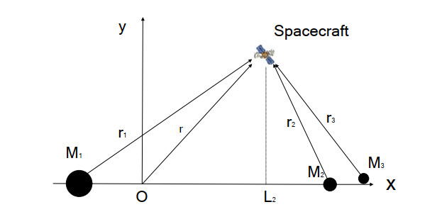
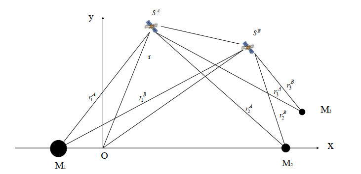
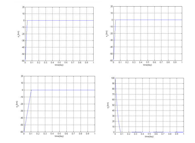
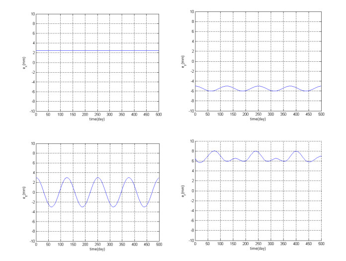
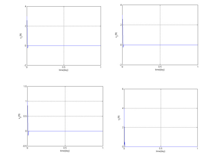
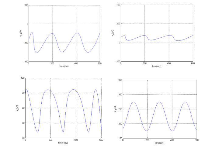
In deep space exploration, the libration points (especially L2 point) of solar-earth system is a re-search hotspot in recent years. Space station and telescope can be arranged at this point, and it does not need too much kinetic energy. Therefore, it is of great significance to arrange flight formation on the libration point of solar-earth for scientific research. However, the flight keeping control technology of flight formation on the solar-earth libration points (also called Lagrange points) is one of the key problems to be solved urgently. Based on the nonlinear dynamic model of formation flying, the improved successive approximation algorithm is used to achieve formation keeping con-trol. Compared with the control algorithm based on orbital elements, this control algorithm has the advantages of high control accuracy and short control time in formation keeping control of solar-earth libration points. The disadvantage is that the calculation is complicated. But, with the devel-opment of computer technology, the computational load is gradually increasing, and there will be more extensive application value in the future. Finally, the error and control simulations of the formation flying of the spacecraft with the libration points of the solar-earth system are carried out for two days. The simulation results show that the method can quickly achieve the requirements of high-precision control.
Citation: Zhenqi He, Lu Yao. Improved successive approximation control for formation flying at libration points of solar-earth system[J]. Mathematical Biosciences and Engineering, 2021, 18(4): 4084-4100. doi: 10.3934/mbe.2021205
In deep space exploration, the libration points (especially L2 point) of solar-earth system is a re-search hotspot in recent years. Space station and telescope can be arranged at this point, and it does not need too much kinetic energy. Therefore, it is of great significance to arrange flight formation on the libration point of solar-earth for scientific research. However, the flight keeping control technology of flight formation on the solar-earth libration points (also called Lagrange points) is one of the key problems to be solved urgently. Based on the nonlinear dynamic model of formation flying, the improved successive approximation algorithm is used to achieve formation keeping con-trol. Compared with the control algorithm based on orbital elements, this control algorithm has the advantages of high control accuracy and short control time in formation keeping control of solar-earth libration points. The disadvantage is that the calculation is complicated. But, with the devel-opment of computer technology, the computational load is gradually increasing, and there will be more extensive application value in the future. Finally, the error and control simulations of the formation flying of the spacecraft with the libration points of the solar-earth system are carried out for two days. The simulation results show that the method can quickly achieve the requirements of high-precision control.

| [1] |
S. Carletta, M. Pontani, P. Teofilatto, Dynamics of three-dimensional capture or-bits from libration region analysis, Acta Astronaut., 165 (2019), 331-343. doi: 10.1016/j.actaastro.2019.09.019

|
| [2] |
G. Pinzari, Perihelion Librations in the Secular Three-Body Problem, J. Nonlinear Sci., 30 (2020), 1771-1808. doi: 10.1007/s00332-020-09624-x
|
| [3] |
S. Wu, Design of interactive digital media course teaching information query system, Inf. Syst. e-Business Manage., 18 (2020), 793-807. doi: 10.1007/s10257-018-00397-1
|
| [4] |
J. Duan, Z. Wang, Orbit determination of CE-4's relay satellite in Earth-Moon L2 libration point orbit, Adv. Space Res., 64 (2019), 2345-2355. doi: 10.1016/j.asr.2019.08.012
|
| [5] | N. Hong, C. T. del Busto, Collaboration, Scaffolding and Successive Approximations: A Developmental Science Approach to Training in Clinical Psychology, Train. Educ. Prof. Psychol., 14 (2020), 228-234. |
| [6] | H. Peng, J. Zhao, Z. Wu, W. Zhong, Optimal periodic controller for formation flying on libration point orbits, Acta Astronaut., 69 (2020), 537-550. |
| [7] |
H. Peng, X. Jiang, B. Chen, Optimal nonlinear feedback control of spacecraft ren-dezvous with finite low thrust between libration orbits, Nonlinear Dyn., 76 (2014), 1611-1632. doi: 10.1007/s11071-013-1233-9
|
| [8] | Y. Jiang, Equilibrium points and orbits around asteroid with the full gravitational potential caused by the 3D irregular shape. Astrodynamics, 14 (2018), 361-373. |
| [9] |
H. Peng, X. Jiang, Nonlinear Receding Horizon Guidance for Spacecraft Formation Re-configuration on Libration Point Orbits using a Symplectic Numerical Method, ISA Trans., 60 (2016), 38-52. doi: 10.1016/j.isatra.2015.10.015
|
| [10] |
R. Chai, A. Tsourdos, A. Savvaris, S. Chai, Y. Xia, C. P. Chen, Six-DOF Spacecraft Optimal Trajectory Planning and Real-Time Attitude Control: A Deep Neural Network-Based Approach, IEEE Trans. Neural Networks Learn. Syst., 31 (2020), 5005-5013. doi: 10.1109/TNNLS.2019.2955400
|
| [11] |
R. Chai, A. Tsourdos, A. Savvaris, S. Chai, Y. Xia, Trajectory planning for hyper-sonic reentry vehicle satisfying deterministic and probabilistic constraints, Acta Astronaut., 177 (2020), 30-38. doi: 10.1016/j.actaastro.2020.06.051
|
| [12] |
W. Zhao, T. Shi, L. Wang, Fault Diagnosis and Prognosis of Bearing Based on Hidden Markov Model with Multi-Features, Appl. Math. Nonlinear Sci., 5 (2020), 71-84. doi: 10.2478/amns.2020.1.00008
|
| [13] |
K. Zhang, Z. He, M. Lv, Study on maintaining formations during satellite formation flying based on SDRE and LQR, Open Phys., 15 (2017), 394-399. doi: 10.1515/phys-2017-0043
|
| [14] |
Y. Zhao, Analysis of Trade Effect in Post-Tpp Era: Based on Gravity Model and Gtap Model, Appl. Math. Nonlinear Sci., 5 (2020), 61-70. doi: 10.2478/amns.2020.1.00007
|
| [15] |
L. Li, Y. Wang, X. Li, Tourists Forecast Lanzhou Based on the Baolan High-Speed Railway by the Arima Model, Appl. Math. Nonlinear Sci., 5 (2020), 55-60. doi: 10.2478/amns.2020.1.00006
|
| [16] |
T. Li, W. Yang, Solution to Chance Constrained Programming Problem in Swap Trailer Transport Organisation based on Improved Simulated Annealing Algorithm, Appl. Math. Nonlinear Sci., 5 (2020), 47-54. doi: 10.2478/amns.2020.1.00005
|
| [17] | Y. Wang, G. Zhang, Z. Shi, Finite-time active disturbance rejection control for marine diesel engine, Appl. Math. Nonlinear Sci., 5 (2020), 35-46. |
| [18] | P. Zhou, Q. Fan, J. Zhu, Empirical Analysis on Environmental Regulation Performance Measurement in Manufacturing Industry: A Case Study of Chongqing, China, Appl. Math. Nonlinear Sci., 5 (2020), 25-34. |
| [19] |
R. A. de Assis, R. Pazim, M. C. Malavazi, A Mathematical Model to describe the herd behaviour considering group defense, Appl. Math. Nonlinear Sci., 5 (2020), 11-24. doi: 10.2478/amns.2020.1.00002
|
| [20] | T. Xie, R. Liu, Z. Wei, Improvement of the Fast Clustering Algorithm Improved by K-Means in the Big Data, Appl. Math. Nonlinear Sci., 5 (2020), 1-10. |
| [21] | B. Shanmukha, V. Venkatesha, Some Results on Generalized Sasakian Space Forms, Appl. Math. Nonlinear Sci., 5 (2020), 85-92. |
| [22] |
M. El-Borhamy, N. Mosalam, On the existence of periodic solution and the transition to chaos of Rayleigh-Duffing equation with application of gyro dynamic, Appl. Math. Nonlinear Sci., 5 (2020), 93-108. doi: 10.2478/amns.2020.1.00010
|
| [23] | H. Günerhan, E. Çelik, Analytical and approximate solutions of Fractional Partial Dif-ferential-Algebraic Equations, Appl. Math. Nonlinear Sci., 5 (2020), 109-120. |
| [24] | T. Li, L. Qiao, Y. Ding, Factors Influencing the Cooperative Relationship between Enterprises in the Supply Chain of China's Marine Engineering Equipment Manufacturing Industry-An study based on GRNN-DEMATEL method, Appl. Math. Nonlinear Sci., 5 (2020), 121-138. |
Figures(6) / Tables(1)

Zhenqi He, Lu Yao. Improved successive approximation control for formation flying at libration points of solar-earth system[J]. Mathematical Biosciences and Engineering, 2021, 18(4): 4084-4100. doi: 10.3934/mbe.2021205


 DownLoad: