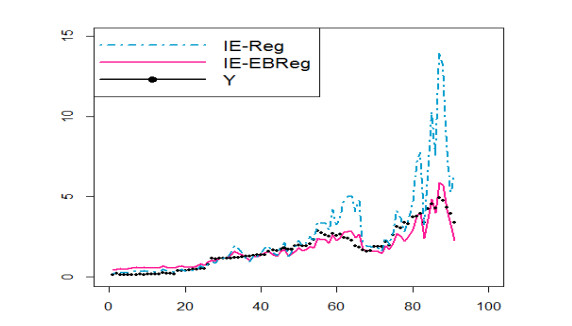
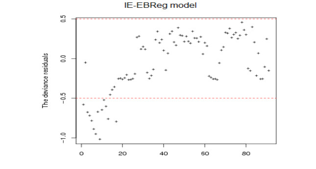
The coronavirus disease 2019 (COVID-19) pandemic caused by the coronavirus strain has had massive global impact, and has interrupted economic and social activity. The daily confirmed COVID-19 cases in Saudi Arabia are shown to be affected by some explanatory variables that are recorded daily: recovered COVID-19 cases, critical cases, daily active cases, tests per million, curfew hours, maximal temperatures, maximal relative humidity, maximal wind speed, and maximal pressure. Restrictions applied by the Saudi Arabia government due to the COVID-19 outbreak, from the suspension of Umrah and flights, and the lockdown of some cities with a curfew are based on information about COVID-15. The aim of the paper is to propose some predictive regression models similar to generalized linear models (GLMs) for fitting COVID-19 data in Saudi Arabia to analyze, forecast, and extract meaningful information that helps decision makers. In this direction, we propose some regression models on the basis of inverted exponential distribution (IE-Reg), Bayesian (BReg) and empirical Bayesian regression (EBReg) models for use in conjunction with inverted exponential distribution (IE-BReg and IE-EBReg). In all approaches, we use the logarithm (log) link function, gamma prior and two loss functions in the Bayesian approach, namely, the zero-one and LINEX loss functions. To deal with the outliers in the proposed models, we apply Huber and Tukey's bisquare (biweight) functions. In addition, we use the iteratively reweighted least squares (IRLS) algorithm to estimate Bayesian regression coefficients. Further, we compare IE-Reg, IE-BReg, and IE-EBReg using some criteria, such as Akaike's information criterion (AIC), Bayesian information criterion (BIC), deviance (D), and mean squared error (MSE). Finally, we apply the collected data of the daily confirmed from March 23 - June 21, 2020 with the corresponding explanatory variables to the theoretical findings. IE-EBReg shows good model for the COVID-19 cases in Saudi Arabia compared with the other models
Citation: Sarah R. Al-Dawsari, Khalaf S. Sultan. Modeling of daily confirmed Saudi COVID-19 cases using inverted exponential regression[J]. Mathematical Biosciences and Engineering, 2021, 18(3): 2303-2330. doi: 10.3934/mbe.2021117
The coronavirus disease 2019 (COVID-19) pandemic caused by the coronavirus strain has had massive global impact, and has interrupted economic and social activity. The daily confirmed COVID-19 cases in Saudi Arabia are shown to be affected by some explanatory variables that are recorded daily: recovered COVID-19 cases, critical cases, daily active cases, tests per million, curfew hours, maximal temperatures, maximal relative humidity, maximal wind speed, and maximal pressure. Restrictions applied by the Saudi Arabia government due to the COVID-19 outbreak, from the suspension of Umrah and flights, and the lockdown of some cities with a curfew are based on information about COVID-15. The aim of the paper is to propose some predictive regression models similar to generalized linear models (GLMs) for fitting COVID-19 data in Saudi Arabia to analyze, forecast, and extract meaningful information that helps decision makers. In this direction, we propose some regression models on the basis of inverted exponential distribution (IE-Reg), Bayesian (BReg) and empirical Bayesian regression (EBReg) models for use in conjunction with inverted exponential distribution (IE-BReg and IE-EBReg). In all approaches, we use the logarithm (log) link function, gamma prior and two loss functions in the Bayesian approach, namely, the zero-one and LINEX loss functions. To deal with the outliers in the proposed models, we apply Huber and Tukey's bisquare (biweight) functions. In addition, we use the iteratively reweighted least squares (IRLS) algorithm to estimate Bayesian regression coefficients. Further, we compare IE-Reg, IE-BReg, and IE-EBReg using some criteria, such as Akaike's information criterion (AIC), Bayesian information criterion (BIC), deviance (D), and mean squared error (MSE). Finally, we apply the collected data of the daily confirmed from March 23 - June 21, 2020 with the corresponding explanatory variables to the theoretical findings. IE-EBReg shows good model for the COVID-19 cases in Saudi Arabia compared with the other models

| [1] | E. Tello-Leal, B. A. Macias-Hernandez, Association of environmental and meteorological factors on the spread of COVID-19 in Victoria, Mexico, and air quality during the lockdown, Environ. Res., (2020), 110442. |
| [2] |
S. Kodera, E. A. Rashed, A. Hirata, Correlation between COVID-19 morbidity and mortality rates in Japan and local population density, temperature, and absolute humidity, Int. J. Env. Res. Pub. He., 17 (2020), 5477. doi: 10.3390/ijerph17155477

|
| [3] | S. A. Meo, A. A. Abukhalaf, A. A. Alomar, N. M. Alsalame, T. Al-Khlaiwi, A. M. Usmani, Effect of temperature and humidity on the dynamics of daily new cases and deaths due to COVID-19 outbreak in Gulf countries in Middle East Region, Eur. Rev. Med. Pharmacol. Sci., 24 (2020), 7524-7533. |
| [4] | L. A. Casado-Aranda, J. Sanchez-Fernandez, M. I. Viedma-del-Jesus, Analysis of the scientific production of the effect of COVID-19 on the environment: A bibliometric study, Environ. Res., (2020), 110416. |
| [5] |
B. Dogan, M. B. Jebli, K. Shahzad, T. H. Farooq, U. Shahzad, Investigating the effects of meteorological parameters on COVID-19: Case study of New Jersey, United States, Environ. Res., 191 (2020), 110148. doi: 10.1016/j.envres.2020.110148
|
| [6] |
S. A. Meo, A. A. Abukhalaf, A. A. Alomar, O. M. Alessa, W. Sami, D. C. Klonoff, Effect of environmental pollutants PM-2.5, carbon monoxide, and ozone on the incidence and mortality of SARS-COV-2 infection in ten wildfire affected counties in California, Sci. Total Environ., 757 (2021), 143948. doi: 10.1016/j.scitotenv.2020.143948
|
| [7] |
J. Yuan, Y. Wu, W. Jing, J. Liu, M. Du, Y. Wang, et al., Non-linear correlation between daily new cases of COVID-19 and meteorological factors in 127 countries, Environ. Res., 193 (2021), 110521. doi: 10.1016/j.envres.2020.110521
|
| [8] | P. McCullagh, J. A. Nelder, Generalized Linear Models, 1$^{st}$ edition, Chapman and Hall, London, 1983. |
| [9] |
J. A. Nelder, D. Pregibon, An extended quasi-likelihood function, Biometrika, 74 (1987), 221-232. doi: 10.1093/biomet/74.2.221
|
| [10] | J. A. Nelder, R. W. M. Wedderburn, Generalized linear models, J. R. Stat. Soc. Ser. A, 135 (1972), 370-384. |
| [11] |
K. H. Yuan, P. M. Bentler, Improving the convergence rate and speed of Fisher-scoring algorithm: ridge and anti-ridge methods in structural equation modeling, Ann. Inst. Stat. Math., 69 (2017), 571-597. doi: 10.1007/s10463-016-0552-2
|
| [12] | P. De Jong, G. Z. Heller, Generalized linear models for insurance data, 1$^{st}$ edition, Cambridge Books, 2008. |
| [13] | T. F. Liao, Interpreting Probability Models: Logit, Probit, and Other Generalized Linear Models, No 07-101, SAGE Publications, Thousand Oaks, 1994. |
| [14] |
R. Richardson, B. Hartman, Bayesian nonparametric regression models for modeling and predicting healthcare claims, Insur. Math. Econ., 83 (2018), 1-8. doi: 10.1016/j.insmatheco.2018.06.002
|
| [15] |
C. Song, Y. Wang, X. Yang, Y. Yang, Z. Tang, X. Wang, et al., Spatial and Temporal Impacts of Socioeconomic and Environmental Factors on Healthcare Resources: A County-Level Bayesian Local Spatiotemporal Regression Modeling Study of Hospital Beds in Southwest China, Int. J. Env. Res. Pub. He., 17 (2020), 5890. doi: 10.3390/ijerph17165890
|
| [16] |
Y. Mohamadou, A. Halidou, P. T. Kapen, A review of mathematical modeling, artificial intelligence and datasets used in the study, prediction and management of COVID-19, Appl. Intell., 50 (2020), 3913-3925. doi: 10.1007/s10489-020-01770-9
|
| [17] | T. A. Trunfio, A. Scala, A. D. Vecchia, A. Marra, A. Borrelli, Multiple Regression Model to Predict Length of Hospital Stay for Patients Undergoing Femur Fracture Surgery at "San Giovanni di Dio e Ruggi d'Aragona" University Hospital, In European Medical and Biological Engineering Conference, Springer, Cham, (2020), 840-847. |
| [18] |
A. Z. Keller, A. R. R. Kamath, U. D. Perera, Reliability analysis of CNC machine tools, Reliab. Eng., 3 (1982), 449-473. doi: 10.1016/0143-8174(82)90036-1
|
| [19] | Y. Abdel-Aty, A. Shafay, M. M. M. El-Din, M. Nagy, Bayesian inference for the inverse exponential distribution based on pooled type-II censored samples, J. Stat. Appl. Pro., 4 (2015), 235. |
| [20] |
S. Dey, Inverted exponential distribution as a life distribution model from a Bayesian viewpoint, Data Sci. J., 6 (2007), 107-113. doi: 10.2481/dsj.6.107
|
| [21] |
S. K. Singh, U. Singh, A. S. Yadav, P. K. Vishwkarma, On the estimation of stress strength reliability parameter of inverted exponential distribution, IJSW, 3 (2015), 98-112. doi: 10.14419/ijsw.v3i1.4329
|
| [22] | L. Fahrmeir, G. Tutz, Multivariate Statistical Modelling Based on Generalized Linear Models, 2$^{nd}$ edition, Springer Science and Business Media, Berlin/Heidelberg, 2013. |
| [23] | E. Cepeda, D. Gamerman, Bayesian methodology for modeling parameters in the two parameter exponential family, Rev. Estad., 57 (2015), 93-105. |
| [24] | D. K. Dey, S. K. Ghosh, B. K. Mallick, Generalized Linear Models: A Bayesian Perspective, 1$^{st}$ edition, CRC Press, New York, 2000. |
| [25] | U. Olsson, Generalized Linear Models, An Applied Approach, 1$^{st}$ edition, Student Litteratur Lund., Sweden, 2002. |
| [26] | N. Sano, H. Suzuki, M. Koda, A robust ensemble learning using zero-one loss function, J. Oper. Res. Soc. Japan, 51 (2008), 95-110. |
| [27] | H. Robbins, An empirical Bayes approach to statistics, In Breakthroughs in statistics, Springer, (1955), 388-394. |
| [28] |
L. Wei, Empirical Bayes test of regression coefficient in a multiple linear regression model, Acta Math. Appl. Sin-E, 6 (1990), 251-262. doi: 10.1007/BF02019151
|
| [29] |
R. S. Singh, Empirical Bayes estimation in a multiple linear regression model, Ann. Inst. Stat. Math., 37 (1985), 71-86. doi: 10.1007/BF02481081
|
| [30] | W. M. Houston, D. J. Woodruff, Empirical Bayes Estimates of Parameters from the Logistic Regression Model, ACT Res. Report Ser., (1997), 97-96. |
| [31] |
S. L. Wind, An empirical Bayes approach to multiple linear regression, Ann. Stat., 1 (1973), 93-103. doi: 10.1214/aos/1193342385
|
| [32] |
S. Y. Huang, Empirical Bayes testing procedures in some nonexponential families using asymmetric Linex loss function, J. Stat. Plan. Infer., 46 (1995), 293-305. doi: 10.1016/0378-3758(94)00112-9
|
| [33] | R. J. Karunamuni, Optimal rates of convergence of empirical Bayes tests for the continuous one-parameter exponential family, Ann. Stat., (1996), 212-231. |
| [34] |
M. Yuan, Y. Lin, Efficient empirical Bayes variable selection and estimation in linear models, J. Am. Stat. Assoc., 100 (2005), 1215-1225. doi: 10.1198/016214505000000367
|
| [35] |
L. S. Chen, Empirical Bayes testing for a nonexponential family distribution, Commun. Stat., Theor. M., 36 (2007), 2061-2074. doi: 10.1080/03610920601143675
|
| [36] | B. Efron, Large-scale inference: Empirical Bayes methods for estimation, testing, and prediction, 1$^{st}$, Cambridge University Press, 2012. |
| [37] | M. Shao, An empirical Bayes test of parameters for a nonexponential distribution family with Negative Quadrant Dependent random samples, In 2013 10th International Conference on Fuzzy Systems and Knowledge Discovery (FSKD), IEEE, (2013), 648-652. |
| [38] |
J. E. Kim, D. A. Nembhard, Parametric empirical Bayes estimation of individual time-pressure reactivity, Int. J. Prod. Res., 56 (2018), 2452-2463. doi: 10.1080/00207543.2017.1380321
|
| [39] |
K. Jampachaisri, K. Tinochai, S. Sukparungsee, Y. Areepong, Empirical Bayes Based on Squared Error Loss and Precautionary Loss Functions in Sequential Sampling Plan, IEEE Access, 8 (2020), 51460-51465. doi: 10.1109/ACCESS.2020.2979872
|
| [40] | Y. Li, L. Hou, Y. Yang, J. Tong, Huber's M-Estimation-Based Cubature Kalman Filter for an INS/DVL Integrated System, Math. Probl. Eng., (2020), 2020. |
| [41] |
B. Sinova, S. Van Aelst, Advantages of M-estimators of location for fuzzy numbers based on Tukey's biweight loss function, Int. J. Approx. Reason., 93 (2018), 219-237. doi: 10.1016/j.ijar.2017.10.032
|
| [42] | P. McCullagh, J. A. Nelder, Generalized Linear Models, 2$^{nd}$ edition, Chapman and Hall/CRC, 1985. |
| [43] |
S. Das, D. K. Dey, On Bayesian analysis of generalized linear models using the Jacobian technique, Am. Stat., 60 (2006), 264-268. doi: 10.1198/000313006X128150
|
| [44] |
S. Ferrari, F. Cribari-Neto, Beta regression for modelling rates and proportions, J. Appl. Stat., 31 (2004), 799-815. doi: 10.1080/0266476042000214501
|
| [45] | S. Das, D. K. Dey, On Bayesian analysis of generalized linear models: A new perspective, Technical Report, Statistical and Applied Mathematical Sciences Institute, Research Triangle Park, (2007), 33. |
| [46] |
P. J. Huber, Robust estimation of a location parameter, Ann. Math. Stat., 35 (1964), 73-101. doi: 10.1214/aoms/1177703732
|
| [47] | P. J. Rousseeuw, A. M. Leroy, Robust Regression and Outlier Detection, 1$^{st}$ edition, John Wiley and Sons, NY, 1987. |
| [48] |
L. Chang, B. Hu, G. Chang, A. Li, Robust derivative-free Kalman filter based on Huber's M-estimation methodology, J. Process Control, 23 (2013), 1555-1561. doi: 10.1016/j.jprocont.2013.05.004
|
| [49] | P. J. Huber, Robust Statistics, 1$^{st}$ edition, John Wiley and Sons, NY, 1981. |
| [50] | R. A. Maronna, R. D. Martin, V. J. Yohai, Robust Statistics: Theory and Methods, 1$^{st}$ edition, John Wiley and Sons, West Sussex, 2006. |
| [51] | F. Wen, W. Liu, Iteratively reweighted optimum linear regression in the presence of generalized Gaussian noise, In 2016 IEEE International Conference on Digital Signal Processing (DSP), IEEE, (2016), 657-661. |
| [52] | H. Kikuchi, H. Yasunaga, H. Matsui, C. I. Fan, Efficient privacy-preserving logistic regression with iteratively Re-weighted least squares, In 2016 11th Asia Joint Conference on Information Security (AsiaJCIS), IEEE, (2016), 48-54. |
| [53] | J. Tellinghuisen, Least squares with non-normal data: Estimating experimental variance functions, Analyst, 133(2) (2008), 161-166. |
| [54] |
R. M. Leuthold, On the use of Theil's inequality coefficients, Am. J. Agr. Econ., 57 (1975), 344-346. doi: 10.2307/1238512
|
| [55] | T. Niu, L. Zhang, B. Zhang, B. Yang, S. Wei, An Improved Prediction Model Combining Inverse Exponential Smoothing and Markov Chain, Math. Probl. Eng., 2020 (2020), 11. |
| [56] | J. J. Faraway, Extending the linear model with R: Generalized linear, mixed effects and nonparametric regression models, 2$^{nd}$ edition, CRC press, 2016. |
| [57] | J. Fox, S. Weisberg, An R companion to applied regression, 3$^rd$ edition, Sage publications, Inc., 2018. |
| [58] | E. Dikici, F. Orderud, B. H. Lindqvist, Empirical Bayes estimator for endocardial edge detection in 3D+ T echocardiography, In 2012 9th IEEE International Symposium on Biomedical Imaging (ISBI), IEEE, (2012), 1331-1334. |
| [59] | A. Coluccia, F. Ricciato, Improved estimation of instantaneous arrival rates via empirical Bayes, In 2014 13th Annual Mediterranean Ad Hoc Networking Workshop, IEEE, (2014), 211-216. |


Figures(6) / Tables(8)

Sarah R. Al-Dawsari, Khalaf S. Sultan. Modeling of daily confirmed Saudi COVID-19 cases using inverted exponential regression[J]. Mathematical Biosciences and Engineering, 2021, 18(3): 2303-2330. doi: 10.3934/mbe.2021117


 DownLoad: