Global dynamics and optimal control of a cholera transmission model with vaccination strategy and multiple pathways

Chenwei Song; Rui Xu; Ning Bai; Xiaohong Tian; Jiazhe Lin; Chenwei Song; Rui Xu; Ning Bai; Xiaohong Tian; Jiazhe Lin

doi:10.3934/mbe.2020233

Mathematical Biosciences and Engineering

2020, Volume 17, Issue 4: 4210-4224. doi: 10.3934/mbe.2020233

Previous Article Next Article

Research article

Global dynamics and optimal control of a cholera transmission model with vaccination strategy and multiple pathways

1.
Complex Systems Research Center, Shanxi University, Taiyuan 030006, Shanxi, P. R. China
2.
Institute of Applied Mathematics, Army Engineering University, Shijiazhuang 050003, Hebei, P. R. China

Received: 01 May 2020 Accepted: 09 June 2020 Published: 15 June 2020

In this paper, we consider a cholera infection model with vaccination and multiple transmission pathways. Dynamical properties of the model are analyzed in detail. It is shown that the disease-free equilibrium is globally asymptotically stable if the basic reproduction number is less than unity; the endemic equilibrium exists and is globally asymptotically stable if the basic reproduction number is greater than unity. In addition, the model is successfully used to fit the real disease situation of cholera outbreak in Somalia. We consider an optimal control problem of cholera transmission with vaccination, quarantine, treatment and sanitation control strategies, and use Pontryagin's minimum principle to determine the optimal control level. The optimal control problem is solved numerically.

Keywords:

Citation: Chenwei Song, Rui Xu, Ning Bai, Xiaohong Tian, Jiazhe Lin. Global dynamics and optimal control of a cholera transmission model with vaccination strategy and multiple pathways[J]. Mathematical Biosciences and Engineering, 2020, 17(4): 4210-4224. doi: 10.3934/mbe.2020233

Related Papers:

[1]	Jiazhe Lin, Rui Xu, Xiaohong Tian . Transmission dynamics of cholera with hyperinfectious and hypoinfectious vibrios: mathematical modelling and control strategies. Mathematical Biosciences and Engineering, 2019, 16(5): 4339-4358. doi: 10.3934/mbe.2019216
[2]	Lili Liu, Xi Wang, Yazhi Li . Mathematical analysis and optimal control of an epidemic model with vaccination and different infectivity. Mathematical Biosciences and Engineering, 2023, 20(12): 20914-20938. doi: 10.3934/mbe.2023925
[3]	Pannathon Kreabkhontho, Watchara Teparos, Thitiya Theparod . Potential for eliminating COVID-19 in Thailand through third-dose vaccination: A modeling approach. Mathematical Biosciences and Engineering, 2024, 21(8): 6807-6828. doi: 10.3934/mbe.2024298
[4]	Zhiping Liu, Zhen Jin, Junyuan Yang, Juan Zhang . The backward bifurcation of an age-structured cholera transmission model with saturation incidence. Mathematical Biosciences and Engineering, 2022, 19(12): 12427-12447. doi: 10.3934/mbe.2022580
[5]	Amira Bouhali, Walid Ben Aribi, Slimane Ben Miled, Amira Kebir . Impact of immunity loss on the optimal vaccination strategy for an age-structured epidemiological model. Mathematical Biosciences and Engineering, 2024, 21(6): 6372-6392. doi: 10.3934/mbe.2024278
[6]	Martin Luther Mann Manyombe, Joseph Mbang, Jean Lubuma, Berge Tsanou . Global dynamics of a vaccination model for infectious diseases with asymptomatic carriers. Mathematical Biosciences and Engineering, 2016, 13(4): 813-840. doi: 10.3934/mbe.2016019
[7]	Tingting Xue, Long Zhang, Xiaolin Fan . Dynamic modeling and analysis of Hepatitis B epidemic with general incidence. Mathematical Biosciences and Engineering, 2023, 20(6): 10883-10908. doi: 10.3934/mbe.2023483
[8]	Jinliang Wang, Ran Zhang, Toshikazu Kuniya . A note on dynamics of an age-of-infection cholera model. Mathematical Biosciences and Engineering, 2016, 13(1): 227-247. doi: 10.3934/mbe.2016.13.227
[9]	Majid Jaberi-Douraki, Seyed M. Moghadas . Optimal control of vaccination dynamics during an influenza epidemic. Mathematical Biosciences and Engineering, 2014, 11(5): 1045-1063. doi: 10.3934/mbe.2014.11.1045
[10]	Linhua Zhou, Meng Fan, Qiang Hou, Zhen Jin, Xiangdong Sun . Transmission dynamics and optimal control of brucellosis in Inner Mongolia of China. Mathematical Biosciences and Engineering, 2018, 15(2): 543-567. doi: 10.3934/mbe.2018025

Abstract

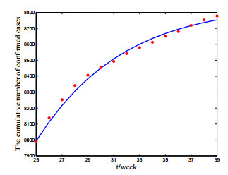
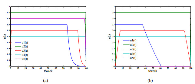
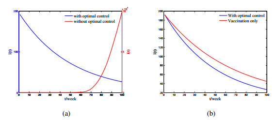
1. Introduction

Cholera is a waterborne disease caused by Vibrio cholera ^[1]. It is well known that it can spread rapidly in countries without clean drinking water and developed public health infrastructure ^[2,3,4]. In 2017, Somalia faced one of the largest outbreaks in history, with 78,784 suspected cases, including 1,159 related deaths. A year later, the number of suspected cases and related deaths reported in Somalia fell due to improved disease surveillance and case management. However, a new cholera outbreak in Somalia began in January 2019 ^[5].

For cholera, the interaction between environment and human is the most common pathway of transmission, that is, human typically is infected by ingesting water or food contaminated by vibrios from the environment ^[6,7,8]. On the other hand, close contacts with infected individuals (such as shaking hands and hugging) can also cause human infection, which indicates that the transmission route of human-to-human also exists ^[9]. A number of studies have shown that human-to-human transmission has a great impact on human infection that can not be ignored ^[10,11,12].

In 2010, Tien et al. formulated a model with multiple pathways ^[13]. It was assumed that the incidence rate is bilinear, indicating that the incidence rate increases with the number of infected individuals and the concentration of vibrio in the environment. However, for environment-to-human transmission, considering the fact that the inhibition effect from behavioral changes of susceptible individuals and the swarming effect of vibrios, the bilinear incidence rate is unreasonable. In 2011, based on the work in ^[13], by introducing a saturation incidence rate $\beta_{1}B /(K+B)$ to describe the inhibition effect, in ^[9], Mukandavire et al. analyzed the following model:

$\begin{equation} \begin{aligned} \dot S& = \mu N-\beta SI-\frac{\beta_{1}S B}{K+B}-\mu S,\\ \dot I& = \beta SI+\frac{\beta_{1}S B}{K+B}-(\gamma+\mu)I,\\ \dot B& = \xi I-\delta B,\\ \dot R& = \gamma I-\mu R,\\ \end{aligned} \end{equation}$

(1.1)

where $S$ , $I$ and $R$ stand for the densities of the susceptible, infected and removed individuals, respectively, and $B$ stands for the concentration of V. cholera in contaminated environment. The parameter $\mu$ denotes the natural birth and death rates of human, $\beta$ and $\beta_{1}$ are the transmission rates of human-to-human and environment-to-human, respectively, $K$ is the pathogen concentration that yields 50% chance of catching cholera, $\gamma$ denotes the recovery rate, $\xi$ is the contribution rate of each infected individual to the concentration of V. cholera shedding from infected individuals and $\delta$ is the net death rate of V. cholerae.

In 2010, WHO recommended the oral vaccines should be used in areas with endemic cholera ^[14]. Subsequently, a number of cholera models with vaccination strategy have been proposed and analysed ^[15,16,17]. In 2015, Posny et al. proposed a new cholera model consisting of vaccination ^[18]. Model analysis shows that the vaccine can effectively control the spread of cholera. However, vaccine protection is not permanent. The existing oral cholera vaccine (OCV) can provide > % continuous protection, lasting for 2 years in the epidemic population ^[14].

Motivated by the works of the WHO report ^[14] and Posny et al. ^[18], in this paper, we focus on the influence of multiple pathways, imperfect vaccination on cholera infection, and analyze the following model:

$\begin{equation} \begin{aligned} \dot S& = A-\mu S-\phi S-\left(\beta I+\frac{\beta_{1}B}{K+B}\right)S +\eta V,\\ \dot V& = \phi S-\left(\beta I+\frac{\beta_{1}B}{K+B}\right)\sigma V-(\mu+\eta)V,\\ \dot I& = \left(\beta I+\frac{\beta_{1}B}{K+B}\right)(S+\sigma V)-(\mu+\gamma+d)I,\\ \dot B& = \xi I-\delta B,\\ \dot R& = \gamma I-\mu R, \end{aligned} \end{equation}$

(1.2)

where $V$ stands for the density of vaccinated individuals. Vaccination rate of susceptible individuals is $\phi$ , vaccine efficiency is $\sigma$ and $1/\eta$ is the duration of vaccine protection. And other parameters have the same biological meanings as in system (1.1).

The initial condition of system (1.2) is

$\begin{equation} \begin{aligned} S(0)\geq0,\quad V(0)\geq0,\quad I(0)\geq0, \quad B(0)\geq0, \quad R(0)\geq0, \end{aligned} \end{equation}$

(1.3)

and we can obtain that all solutions of system (1.2) remain positive for all $t \geq 0$ .

The organization of this paper is as follows. In Section 2, we show the existence of feasible equilibria. In Section 3, we establish the global stability of each of feasible equilibria of system (1.2) by constructing Liapunov functions. In Section 4, we consider the optimal control problem of cholera model with vaccination, quarantine, treatment and sanitation control strategies. In order to determine the optimal control strategy, we use Pontryagin's minimum principle. In Section 5, the model is used to fit the real disease situation of cholera outbreak in Somalia. Besides, we analyze the sensitivity of the basic reproduction number and solve the resulting optimality problem numerically. Finally, a brief discussion is given in Section 6 to end this work.

2. Equilibria and boundedness of solutions

For system (1.2), it is easy to conclude that there is always a disease-free equilibrium $E_{0}(S_{0}, V_{0}, 0, 0, 0)$ , where

$S_{0} = \frac{A(\mu+\eta)}{\mu(\mu+\eta+\phi)}, \quad V_{0} = \frac{A\phi}{\mu(\mu+\eta+\phi)}.$

Below, we first calculate the basic reproduction number $R_{0}$ by using the method of the next generation matrix ^[19]. Let

$\begin{gathered} \mathcal{F} = \left( \begin{array}{c} \left(\beta I+\frac{\beta_{1}B}{K+B}\right)(S+\sigma V)\\ 0 \\ \end{array} \right), \quad \mathcal{V} = \left(\begin{array}{c} (\mu+\gamma+d)I\\ -\xi I+\delta B \\ \end{array} \right). \end{gathered}$

Computing the Jacobian Matrix at $E_{0}$ , we have

$\begin{aligned} F = \begin{pmatrix} \beta S_{0}+\sigma \beta V_{0} & \frac{\beta_{1} S_{0}+\sigma \beta_{1} V_{0}}{K}\\ 0 & 0\\ \end{pmatrix}, \quad V = \begin{pmatrix} \mu+\gamma+d & 0 \\ -\xi & \delta\\ \end{pmatrix}. \end{aligned}$

It follows that

$\begin{gathered} FV^{-1} = \begin{pmatrix} \frac{\beta S_{0}+\sigma \beta V_{0}}{\mu+\gamma+d }+\frac{(\beta_{1} S_{0}+\sigma\beta_{1} V_{0})\xi}{K\delta(\mu+\gamma+d )}& \frac{\beta_{1} S_{0}+\sigma \beta_{1} V_{0}}{K\delta}\\ 0 & 0\\ \end{pmatrix}. \end{gathered}$

We obtain:

$R_{0} = \frac{A\beta(\mu+\eta+\sigma\phi) }{\mu (\mu+\gamma+d)(\mu+\eta+\phi)}+\frac{A\beta_{1}\xi(\mu+\eta+\sigma\phi)}{\mu K \delta(\mu+\gamma+d)(\mu+\eta+\phi)}.$

If $R_{0} > 1$ , system (1.2) has a disease-free equilibrium $E_{0}(S_{0}, V_{0}, 0, 0, 0)$ and an endemic equilibrium $E^{*}(S^{*}, V^{*}, I^{*}, B^{*}, R^{*})$ , where

$\begin{aligned} S^{*}& = \frac{a_{0}(K+B^{*})^{2}+a_{1}(K+B^{*})}{ a_{2}(K+B^{*})^{2}+a_{3}(K+B^{*})+a_{4}},\; V^{*} = \frac{A\phi\xi^{2}(K+B^{*})^{2}}{a_{2}(K+B^{*})^{2}+a_{3}(K+B^{*})+a_{4}},\\ I^{*}& = \frac{\delta}{\xi}B^{*},\quad\quad\quad\quad \quad \quad R^{*} = \frac{\gamma \delta}{\mu \xi}B^{*},\\ \end{aligned}$

here

$\begin{aligned} a_{0}& = A(\mu+\eta)\xi^{2},\quad \quad\quad\quad \\ a_{1}& = A\xi\sigma B^{*}(\delta\beta+\beta_{1}\xi),\\ a_{2}& = \beta\delta B^{*}[\sigma\delta\beta B^{*}+(\mu+\eta)\xi]+(\phi+\mu+\eta)\mu,\\ a_{3}& = \sigma\beta_{1}B^{*}\xi[\beta\delta B^{*}+(\phi+\mu)\xi]+\beta_{1} B^{*}\xi[\sigma\delta\beta B^{*}+(\mu+\eta)\xi],\\ a_{4}& = \sigma\beta_{1}^{2}B^{*2}\xi^{2}, \end{aligned}$

and $B^{*}$ is the positive real root of the equation $h(B) = 0$ , where

$\begin{equation} \begin{aligned} h(B) = b_{4}B^{4}+b_{3}B^{3}+b_{2}B^{2}+b_{1}B+b_{0}, \end{aligned} \end{equation}$

(2.1)

in which

$\begin{aligned} b_{0} = &k^{2}\delta\mu\xi^{2}(\mu+\gamma+d)(\mu+\phi+\eta)(1-R_{0}),\\ b_{1} = &(\mu+\gamma+d)[K^{2}\beta\delta^{2}(\mu+\eta)\xi+K^{2}\beta\sigma\delta^{2}(\phi+\mu)\xi +2K\delta\mu(\mu+\phi+\eta)\xi^{2}\\ &+K\delta\beta_{1}\xi^{2}(\mu+\eta)+K\sigma\delta\beta_{1}\xi^{2}(\mu+\phi)] -K^{2}A\xi\beta^{2}\sigma\delta^{2}-2KA\xi^{2}\beta\delta(\mu+\eta+\phi\sigma)\\ &-2KA\beta\beta_{1}\xi^{2}\sigma\delta-A\xi^{3}\beta_{1}(\mu+\eta+\phi\sigma) -A\xi^{3}\beta_{1}^{2}\sigma,\\ b_{2} = &(\mu+\gamma+d)[K^{2}\beta^{2}\sigma\delta^{3}+2K\beta\delta^{2}(\mu+\eta)\xi +2K\beta\sigma\delta^{2}(\phi+\mu)\xi+\delta\mu(\mu+\phi+\eta)\xi^{2}\\ &+2K\xi\beta\beta_{1}\sigma\delta^{2}+(\phi+\mu)\xi^{2}\beta_{1}\delta\sigma +\beta_{1}\delta\xi^{2}(\mu+\eta)+\sigma\beta_{1}^{2}\delta\xi^{2}]-2kA\xi\beta^{2}\sigma\delta^{2}\\ &-2A\xi^{2}\beta\beta_{1}\delta\sigma-A\beta\delta\xi^{2}(\mu+\eta+\phi\sigma),\\ b_{3} = &(\mu+\gamma+d)[2K\beta^{2}\sigma\delta^{3}+\beta\delta^{2}(\mu+\eta)\xi +\beta\sigma\delta^{2}(\phi+\mu)\xi+2\beta\beta_{1}\sigma\delta^{2}\xi]-A\xi\sigma\beta^{2}\delta^{2},\\ b_{4} = &(\mu+\gamma+d)\beta^{2}\sigma\delta^{3}.\\ \end{aligned}$

Note that $\lim_{B\rightarrow+\infty}h(B) = +\infty$ , $h(0) = b_0 < 0$ if $R_{0} > 1$ , in this case, system (1.2) has a positive equilibrium $E^{*}$ .

Let $N = S+V+I+R.$ Then $\dot{N} = A-\mu(S+V+I+R)-dI \leq A-\mu N$ . It follows that

$\limsup\limits_{t\rightarrow+\infty} N(t)\leq A/\mu.$

Furthermore, we derive from the fourth equation of system (1.2),

$\limsup\limits_{t\rightarrow+\infty} B(t)\leq A\xi/\mu\delta.$

We therefore conclude that the set

$\Omega = \left\{(S, V, I, B, R)\in R_{+}^{5}: 0 \leq S(t)+V(t)+I(t)+R(t)\leq\frac{A}{\mu}, 0 \leq B(t)\leq\frac{A\xi}{\mu\delta} \right\}$

is positively invariant.

3. Global stability

In this section, we study the global stability of each of the equilibria to system (1.2). The approach of proofs is to use suitable Lyapunov function.

Theorem 3.1. If $R_{0} < 1$ , the disease-free equilibrium $E_{0}(S_{0}, V_{0}, 0, 0, 0)$ of system (1.2) is globally asymptotically stable.

Proof. Define

$\begin{aligned} W(t)& = S_{0}\left(\frac{S}{S_{0}}-1-\ln\frac{S}{S_{0}}\right)+V_{0}\left(\frac{V}{V_{0}}-1-\ln\frac{V}{V_{0}}\right)+I+\frac{\beta_{1}S_{0}+\sigma \beta_{1}V_{0}}{K\delta}B.\\ \end{aligned}$

Calculating the derivative of $W(t)$ along positive solutions of system (1.2), one has

$\begin{equation} \begin{aligned} \dot{W}(t)& = \left(1-\frac{S_{0}}{S}\right)\left(A-\mu S-\phi S-\left(\beta I+\frac{\beta_{1}B}{K+B}\right)S+\eta V\right)\\ &+\left(1-\frac{V_{0}}{V}\right)\left(\phi S-\left(\beta I+\frac{\beta_{1}B}{K+B}\right)\sigma V-(\mu+\eta)V\right)\\ &+\left(\beta I+\frac{\beta_{1}B}{K+B}\right)(S+\sigma V)-(\mu+\gamma+d)I\\ &+\frac{\beta_{1}S_{0}+\sigma \beta_{1}V_{0}}{K\delta}(\xi I-\delta B). \end{aligned} \end{equation}$

(3.1)

On substituting $A = \mu S_{0}+\mu V_{0}$ , $\phi S_{0} = (\mu + \eta)V_{0}$ into (3.1), we obtain that

$\begin{aligned} \dot{W}(t)& = \mu S_{0}\left(2-\frac{S_{0}}{S}-\frac{S}{S_{0}}\right)+\eta V_{0}\left(2-\frac{S_{0}V}{V_{0}S}-\frac{V_{0}S}{S_{0}V}\right)\\ &{+\mu V_{0}\left(3-\frac{S}{S_{0}}-\frac{V}{V_{0}}-\frac{V_{0}S}{S_{0}V}\right) +(\mu+\gamma+d)\left(R_{0}-1\right)I}\\ &-\frac{(\beta_{1}S_{0}+\sigma \beta_{1}V_{0})B^{2}}{K(K+B)}\leq0, \end{aligned}$

and $\dot{W}(t) < 0$ for all $(S, V, I, B, R)\neq(S_{0}, V_{0}, 0, 0, 0)$ . Therefore, by Lyapunov's stability Theorem ^[20], the equilibrium $E_{0}$ is globally asymptotically stable.

Theorem 3.2. If $R_{0} > 1$ , the endemic equilibrium $E^{*}(S^{*}, V^{*}, I^{*}, B^{*}, R^{*})$ of system (1.2) is globally asymptotically stable.

Proof. Define

$\begin{aligned} W_{1}(t)& = S^{*}\left(\frac{S}{S^{*}}-1-\ln\frac{S}{S^{*}}\right)+V^{*}\left(\frac{V}{V^{*}}-1-\ln\frac{V}{V^{*}}\right)\\ &+I^{*}\left(\frac{I}{I^{*}}-1-\ln\frac{I}{I^{*}}\right)+\frac{\beta_{1}S^{*}+\sigma\beta_{1}V^{*}}{(K+B^{*})\delta} B^{*}\left(\frac{B}{B^{*}}-1-\ln\frac{B}{B^{*}}\right).\\ \end{aligned}$

Calculating the derivative of $W_{1}(t)$ along positive solutions of system (1.2), one has

$\begin{equation} \begin{aligned} \dot{W_{1}}(t)& = \left(1-\frac{S^{*}}{S}\right)\left(A- \mu S-\phi S-\left(\beta I+\frac{\beta_{1}B}{K+B}\right)S+\eta V\right)\\ &+\left(1-\frac{V^{*}}{V}\right)\left(\phi S-\left(\beta I+\frac{\beta_{1}B}{K+B}\right)\sigma V-(\mu+\eta)V\right)\\ &+\left(1-\frac{I^{*}}{I}\right)\left(\left(\beta I+\frac{\beta_{1}B}{K+B}\right)(S+\sigma V)-(\mu+\gamma+d)I\right)\\ &+\frac{\beta_{1}S^{*}+\sigma\beta_{1}V^{*}}{(K+B^{*})\delta}\left(1-\frac{B^{*}}{B}\right)(\xi I-\delta B). \end{aligned} \end{equation}$

(3.2)

On substituting

$\begin{aligned} &A = (S^{*}+\sigma V^{*})\left(\beta I^{*}+\frac{\beta_{1}B^{*}}{K+B^{*}}\right)+\mu S^{*}+\mu V^{*},\\ &\phi S^{*} = \sigma V^{*}\left(\beta I^{*}+\frac{\beta_{1}B^{*}}{K+B^{*}}\right)+(\mu+\eta) V^{*},\\ &(\mu+\gamma+d)I^{*} = (S^{*}+\sigma V^{*})\left(\beta I^{*}+\frac{\beta_{1}B^{*}}{K+B^{*}}\right),\\ &\delta B^{*} = \xi I^{*} \end{aligned}$

into (3.2), we have

$\begin{aligned} \dot{W_{1}}(t)& = (\mu+\beta I^{*}) S^{*}\left(2-\frac{S}{S^{*}}-\frac{S^{*}}{S}\right) +\eta V^{*}\left(2-\frac{S^{*}V}{V^{*}S}-\frac{V^{*}S}{S^{*}V}\right)\\ &+(\mu+\sigma\beta I^{*}) V^{*}\left(3-\frac{S^{*}}{S}-\frac{V}{V^{*}}-\frac{V^{*}S}{S^{*}V}\right)\\ &+\frac{\beta_{1}S^{*}B^{*}}{K+B^{*}}\left(4-\frac{S^{*}}{S}-\frac{B^{*}I}{I^{*}B} -\frac{K+B}{K+B^{*}}-\frac{(K+B^{*})I^{*}SB}{S^{*}B^{*}(K+B)I}\right)\\ &+\frac{\sigma\beta_{1} V^{*}B^{*}}{K+B^{*}}\left(5-\frac{S^{*}}{S}-\frac{V^{*}S}{S^{*}V} -\frac{B^{*}I}{I^{*}B}-\frac{K+B}{K+B^{*}}-\frac{(K+B^{*})I^{*}VB}{V^{*}B^{*} (K+B)I}\right)\\ &-\frac{K\beta_{1}(S^{*}+\sigma V^{*})(B^{*}-B)^{2}}{(K+B^{*})^{2}(K+B)}\leq0, \end{aligned}$

and $\dot{W_{1}}(t) < 0$ for all $(S, V, I, B, R)\neq(S^{*}, V^{*}, I^{*}, B^{*}, R^{*})$ . Therefore, by Lyapunov's stability Theorem ^[20], the equilibrium $E^{*}$ is globally asymptotically stable.

4. Optional control strategies

We consider the optimal control problem of cholera model with vaccinate, quarantine, treatment and sanitation control strategies:

$\begin{equation} \begin{aligned} \dot S& = A-(\mu+u_{1}(t)) S-\left(\beta(1-u_{2}(t))I+\frac{\beta_{1}(1-u_{3}(t))B}{K+B}\right)S+\eta V,\\ \dot V& = u_{1}(t)S-\left(\beta (1-u_{2}(t))I+\frac{ \beta_{1}(1-u_{3}(t))B}{K+B}\right)\sigma V-(\mu+\eta)V,\\ \dot I& = \left(\beta(1-u_{2}(t))I+\frac{\beta_{1}(1-u_{3}(t))B}{K+B}\right)(S+\sigma V)-(\mu+d+\gamma+u_{4}(t))I,\\ \dot B& = \xi I-(\delta+u_{5}(t)) B,\\ \dot R& = (\gamma+u_{4}(t))I-\mu R.\\ \end{aligned} \end{equation}$

(4.1)

Where $u_{1}(t)$ is a vaccination strategy aimed to the susceptible individuals; $u_{2}(t)$ is a quarantine strategy that can reduce the transmission of human-to-human; $u_{3}(t)$ is another kind of quarantine strategy that can reduce the transmission of environment-to-human; $u_{4}(t)$ is therapeutic treatment aimed to the infected people, $u_{5}(t)$ is a sanitation strategy aimed at killing vibrios in contaminated water.

Define a control function set as $\textbf{U} = \{u_{i}(t)\mid i = 1, \cdots, 5\},$ and $\textbf{X} = (S, V, I, B, R).$ The admissible trajectories of set $\mathcal{\textbf{X}}$ are given by

$\mathcal{X} = \{\textbf{X}(.)\in W^{1,1}([0,T);R^{5})\mid\;(1.3)\; \rm{and}\;(4.1)\; \rm{are\; satisfied}\}.$

Define

$\mathcal{U} = \{\textbf{U}(\cdot)\in L^{\infty}([0,T];R^{5})\;| 0\leq u_{i}(t)\leq u_{imax}\leq1,\;i = 1,\cdots,5, \; {\forall}\;t\;\in[0,T]\},$

where $u_{imax}\; (i = 1, \cdots, 5)$ denote the upper bounds for the efforts of vaccination, quarantine strategy, another kind of quarantine strategy, treatment and sanitation, respectively.

The objective functional

$\begin{aligned} &Q(\textbf{X}(\cdot),\textbf{U}(\cdot)) = \int_{0}^{T}g(\textbf{X}(t),\textbf{U}(t))dt.\\ \end{aligned}$

The function $g$ is called the running payoff function ^[20]. The objective of the optimal control problem is to minimize the objective functional

$\begin{equation} \begin{aligned} Q(\textbf{X}^{*}(\cdot),\textbf{U}^{*}(\cdot)) = \min\limits_{\textbf{X}(\cdot),\textbf{U}(\cdot) \in\mathcal{X}\times\mathcal{U}}Q(\textbf{X}(\cdot),\textbf{U}(\cdot)). \end{aligned} \end{equation}$

(4.2)

The first question that must be addressed is the existence of the optimal control pair. According to the Filippov-Cesari existence theorem ^[20], we obtain the following result.

Theorem 4.1. There exists a $\boldsymbol{U}^{*}(\cdot)$ such that the objective functional in (4.2) is minimized.

To apply Pontryagin's minimum principle ^[21], we need to introduce the adjoint vector function $\lambda(t) = (\lambda_{S}(t), \lambda_{I}(t), \lambda_{V}(t), \lambda_{B}(t), \lambda_{R}(t)),$ to define the Hamiltonian:

$\begin{aligned} H(\textbf{X},\textbf{U},\lambda)& = g(\textbf{X}(t),\textbf{U}(t))\\ &+\lambda_{S}\left(A-(\mu+u_{1}(t)) S-\left(\beta(1-u_{2}(t))I+\frac{\beta_{1}(1-u_{3}(t))B}{K+B}\right)S+\eta V\right)\\ &+\lambda_{V}\left(u_{1}(t)S- \left(\beta (1-u_{2}(t))I+\frac{ \beta_{1}(1-u_{3}(t))B}{K+B}\right)\sigma V-(\mu +\eta)V\right)\\ &+\lambda_{I}\left[\left(\beta(1-u_{2}(t))I+\frac{\beta_{1}(1-u_{3}(t))B}{K+B}\right)(S +\sigma V)-(\mu+d+\gamma+u_{4}(t))I\right]\\ &+\lambda_{B}\left[\xi I-(\delta+u_{5}(t))B\right]\\ &+\lambda_{R}\left[(\gamma+u_{4}(t))I-\mu R\right]. \end{aligned}$

The adjoint functions must satisfy

$\lambda_{S}^{'} = -\frac{\partial H}{\partial S},\quad \lambda_{V}^{'} = -\frac{\partial H}{\partial V},\quad \lambda_{I}^{'} = -\frac{\partial H}{\partial I}, \quad \lambda_{B}^{'} = -\frac{\partial H}{\partial B}, \quad \lambda_{R}^{'} = -\frac{\partial H}{\partial R}.$

That is,

$\begin{equation} \begin{aligned} \frac{d\lambda_{S}}{dt}& = (\mu+u_{1}(t))\lambda_{S} +\left(\beta(1-u_{2}(t))I+\frac{\beta_{1}(1-u_{3}(t))B}{K+B}\right)(\lambda_{S}-\lambda_{I}) -u_{1}(t)\lambda_{V}-\frac{\partial g}{\partial S}\\ \frac{d\lambda_{V}}{dt}& = (\mu+\eta)\lambda_{V}+\left(\sigma\beta(1-u_{2}(t))I +\frac{\sigma\beta_{1}(1-u_{3}(t))B}{K+B}\right)(\lambda_{V}-\lambda_{I})-\eta\lambda_{S}-\frac{\partial g}{\partial V},\\ \frac{d\lambda_{I}}{dt}& = \beta(1-u_{2}(t))S(\lambda_{S}-\lambda_{I})+ \sigma\beta(1-u_{2}(t))V(\lambda_{V}-\lambda_{I})+(\mu+\gamma+u_{4}(t)+d)\lambda_{I}\\ &-\xi\lambda_{B}-u_{4}(t)\lambda_{R}-\frac{\partial g}{\partial I},\\ \frac{d\lambda_{B}}{dt}& = \frac{\beta_{1}(1-u_{3}(t))S K}{(K+B)^{2}}(\lambda_{S}-\lambda_{I})+\frac{\sigma\beta_{1}(1-u_{3}(t))V K}{(K+B)^{2}}(\lambda_{V}-\lambda_{I})+(\delta+u_{5}(t))\lambda_{B}-\frac{\partial g}{\partial B},\\ \frac{d\lambda_{R}}{dt}& = \mu\lambda_{R}-\frac{\partial g}{\partial R}, \end{aligned} \end{equation}$

(4.3)

with transversality condition

$\begin{equation} \begin{aligned} \lambda_{S}(T) = \lambda_{V}(T) = \lambda_{I}(T) = \lambda_{B}(T) = \lambda_{R}(T) = 0, \quad j = 1, 2. \end{aligned} \end{equation}$

(4.4)

Moreover, the characterizations of the optimal controls are based on

$\begin{aligned} \frac{\partial H}{\partial u_{i}} = 0, \quad \quad\quad\;\; i = 1,\cdots,5. \end{aligned}$

In order to explore the sensitivity of the cost function to the optimal control solution, we consider two different cost functions for the running payoff function $g(\textbf{X}(t), \textbf{U}(t))$ . If we choose the running payoff function

$\begin{equation} \begin{aligned} g_{1}(\textbf{X}(t),\textbf{U}(t)) = I+\frac{C_{11}}{2}u_{1}(t)^{2}+\frac{C_{21}}{2}u_{2}(t)^{2} +\frac{C_{31}}{2}u_{3}(t)^{2}+\frac{C_{41}}{2}u_{4}(t)^{2}+\frac{C_{51}}{2}u_{5}(t)^{2}, \end{aligned} \end{equation}$

(4.5)

where $C_{i1}(i = 1, \cdots, 5)$ are the weight constants for the control strategies. The $C_{11}u_{1}^{2}/2$ , $C_{21}u_{2}^{2}/2$ , $C_{31}u_{3}^{2}/2$ , $C_{41}u_{4}^{2}/2$ , $C_{51}u_{5}^{2}/2$ define the appropriate costs function associated with these controls ^[20]. We can obtain that

$\begin{equation} \begin{aligned} \widetilde{u}_{11}& = \frac{(\lambda_{S1}-\lambda_{V1})S}{C_{11}}, \quad \widetilde{u}_{21} = \frac{\beta SI(\lambda_{I1}-\lambda_{S1})+\sigma\beta VI(\lambda_{I1}-\lambda_{V1})}{C_{21}},\\ \widetilde{u}_{31}& = \frac{\beta_{1} SB(\lambda_{I1}-\lambda_{S1})+\sigma\beta_{1} VB(\lambda_{I1}-\lambda_{V1})}{C_{31}(K+B)},\quad \widetilde{u}_{41} = \frac{(\lambda_{I1}-\lambda_{R1})I}{C_{41}},\\ \widetilde{u}_{51}& = \frac{\lambda_{B1}B}{C_{51}}. \end{aligned} \end{equation}$

(4.6)

In addition, if we choose another running payoff function

$\begin{equation} \begin{aligned} g_{2}(\textbf{X}(t),\textbf{U}(t))& = I+C_{12}\left(u_{1}(t)+u_{1}(t)^{2}\right)+C_{22}\left(u_{2}(t)+u_{2}(t)^{2}\right)+C_{32}\left(u_{3}(t)+u_{3}(t)^{2}\right)\\ &+C_{42}\left(u_{4}(t)+u_{4}(t)^{2}\right)+C_{52}\left(u_{5}(t)+u_{5}(t)^{2}\right), \end{aligned} \end{equation}$

(4.7)

where $C_{i2}(i = 1, \cdots, 5)$ are the weight constants for the control strategies. $C_{12}\left(u_{1}(t)+u_{1}(t)^{2}\right)$ , $C_{22}\left(u_{2}(t)+u_{2}(t)^{2}\right)$ , $C_{32}\left(u_{3}(t)+u_{3}(t)^{2}\right)$ , $C_{42}\left(u_{4}(t)+u_{4}(t)^{2}\right)$ , $C_{52}\left(u_{5}(t)+u_{5}(t)^{2}\right)$ define the appropriate costs function associated with these controls ^[23]. We can obtain that

$\begin{equation} \begin{aligned} \widetilde{u}_{12}& = \frac{(\lambda_{S2}-\lambda_{V2})S-C_{12}}{2C_{12}}, \quad \widetilde{u}_{22} = \frac{\beta SI(\lambda_{I2}-\lambda_{S2})+\sigma\beta VI(\lambda_{I2}-\lambda_{V2})-C_{22}}{2C_{22}},\\ \widetilde{u}_{32}& = \frac{\beta_{1} SB(\lambda_{I2}-\lambda_{S2})+\sigma\beta_{1} VB(\lambda_{I2}-\lambda_{V2})-C_{32}}{2C_{32}(K+B)},\quad \widetilde{u}_{42} = \frac{(\lambda_{I2}-\lambda_{R2})I-C_{42}}{C_{42}},\\ \widetilde{u}_{52}& = \frac{\lambda_{B2}B-C_{52}}{2C_{52}}. \end{aligned} \end{equation}$

(4.8)

Where $\lambda_{Sj}, \lambda_{Vj}, \lambda_{Ij}, \lambda_{Bj}, \lambda_{Rj}(j = 1, 2)$ satisfy the equations (4.3) and (4.4). Based on this fact, we obtain $\widetilde{u}_{ij}(i = 1, \cdots, 5, j = 1, 2)$ . Further, we have

$u_{ij}^{*} = \max[0,\min(\widetilde{u}_{ij},u_{imax})].$

Next, in Section 5, we apply the forward-backward sweep method to solve it numerically ^[15,20].

5. Numerical simulations

In this section, system (1.2) is used to fit the real disease situation of cholera outbreak in Somalia. Besides, we analyze the sensitivity of $R_{0}$ . As mentioned in Section 4, the optimal control problem needs to be solved by numerical simulation, we will show the numerical result. In addition, we list the values of parameters in Table 1.

Table 1. Table of biologically relevant parameter values (week).

Parameter	Description	Value	Source
$A$	Constant birth rate	7342	^[5]
$\phi$	Vaccinate rate of susceptible	$4.2836\times10^{-3}$	fitting
$\beta$	Transmission rate of human-to-human	$4.3771\times10^{-10}$	fitting
$\beta_1$	Transmission rate of environment-to-human	$0.5959\times10^{-4}$	fitting
$K$	Concentration of V. cholera in environment	$10^{6}$	^[8]
$\mu$	Natural death rate of human	0.00038	^[5]
$\eta$	Waning rate of vaccinate	0.0104	^[14]
$\sigma$	Reduction rate of vaccine efficacy	0.5	^[14]
$\gamma$	Recovery rate of infected individuals	1.5	^[8]
$d$	Cholera mortality	0.006	^[5]
$\xi$	Rate of release of V. cholerae	70	^[8]
$\delta$	Natural death rate of V. cholera	0.197	^[8]
Initial values	Description	Value	Source
$S(0)$	Initial susceptible population	12316000	^[22]
$V(0)$	Initial vaccinated population	0	^[22]
$I(0)$	Initial infected population	$192$	^[22]
$B(0)$	Initial concentration of vibrios	$205740$	fitting
$R(0)$	Initial recovered population	$147$	fitting

| Show Table

DownLoad: CSV

5.1. Data fitting

In this subsection, we use system (1.2) to fit the real disease situation of cholera outbreak in Somalia. The new cholera outbreak in Somalia began in January 2019, and the first round of oral cholera vaccination (OCV) activity started on June 22, 2019, the 25th week of 2019, so our numerical simulation starts from the 25th week of 2019.

In addition, the data we obtained is the cumulative number of cases since December 2017, so our initial case number is 7,994 ^[22]. By using the Markov Chain Monte Carlo method, we can get fitting results (see Figure 1). It is shown that the solutions of system (1.2) are in good agreement with the actual cholera cases, which verifies the rationality of the model established in this paper.

Figure 1. Cumulative cases in Somalia between weeks 25 and 39 of 2019, in which the red dots represent the reported data, the blue curve is the solution of model (1.2).

DownLoad: Full-Size Img PowerPoint

5.2. Sensitivity analysis

In this subsection, we use the Latin hypercube sampling (LHS) method to analyze the sensitivity of $R_{0}$ ^[24]. Through the analysis of LHS samples, we obtain the Partial Rank Correlation Coefficients (PRCC) with respect to $R_{0}$ (see ). It is easy to see that $\beta_{1}, \xi, \eta, \beta, \sigma$ are positive correlative variables with $R_{0}$ ; and $\phi, \gamma$ are negative correlative variables with $R_{0}$ .

Figure 2. Tornado plot of partial rank correlation coefficients in respect to

$R_{0}$ .

DownLoad: Full-Size Img PowerPoint

5.3. Optimal control solution

In this subsection, we will show the optimal control results. Based on empirical values, we set $u_{1max} = 0.7, u_{2max} = 0.9, u_{3max} = 0.6, u_{4max} = 0.5, u_{5max} = 0.8$ , respectively. Meanwhile, we assume that the costs for vaccination, treatment, quarantine and sanitation per unit of time is roughly the same.

We first consider the running payoff function $g_{1}(\textbf{X}(t), \textbf{U}(t))$ . The following set of values for the cost parameters

$\begin{equation*} \label{51} \begin{split} C_{11} = 1,\quad C_{21} = 1,\quad C_{31} = 1,\quad C_{41} = 1, \quad C_{51} = 1. \end{split} \tag{5.1} \end{equation*}$

(5.1)

The optimal control solution is shown in . The vaccination strategy $u_{1}(t)$ can be reduced 80 weeks later from the beginning of the cholera break, and the quarantine strategy $u_{2}(t)$ , treatment strategy $u_{4}(t)$ and sanitation strategy $u_{5}(t)$ should be maintained in the whole process. Another quarantine strategy $u_{3}(t)$ should be gradually increased over 1 weeks and maintained at a high level until 90 weeks.

Figure 3. The graph trajectories of five optimal control strategies based on different running payoff function, in which (a)

$g_{1}(\textbf{X}(t), \textbf{U}(t))$ with the cost parameter (5.1), (b)

$g_{2}(\textbf{X}(t), \textbf{U}(t))$ with the cost parameter (5.2).

DownLoad: Full-Size Img PowerPoint

Next, we consider the running payoff function $g_{2}(\textbf{X}(t), \textbf{U}(t))$ . The following set of values for the cost parameters

$\begin{equation*} \label{52} \begin{split} C_{12} = 1,\quad C_{22} = 1,\quad C_{32} = 1,\quad C_{42} = 1, \quad C_{52} = 1. \end{split} \tag{5.2} \end{equation*}$

(5.2)

Similarly, the optimal control solution is shown in . The vaccination strategy $u_{1}(t)$ can be reduced 40 weeks later from the beginning of the cholera break, and the quarantine strategy $u_{2}(t)$ , treatment strategy $u_{4}(t)$ should be maintained in the whole process. Another quarantine strategy $u_{3}(t)$ should be gradually increased over 10 weeks and maintained at a high level until 90 weeks. In addition, the sanitation strategy $u_{5}(t)$ is not recommended.

As shown in Figure 3, the values obtained on the optimal control analysis is sensitive to the selected cost function. Therefore, there are different optimal control measures when considering different cost functions. Further, based on the optimal control measures, we can get the effects of the control strategies for the infected individuals. In order to make a comparison, we consider the effects of without any control measures (see Figure 4(a), Figure 5(a)). It is well known that vaccination is a effective measure for cholera prevention and control in a short term. In the following, we explore the influence of vaccine control alone for the infected individuals (see Figure 4(b), Figure 5(b)). By Figure 4 and Figure 5, we can conclude that combining multiple control strategies are most likely to yield the best results in fighting cholera, and the vaccine has a significant control effect on cholera.

Figure 4. The graph trajectories of

$I(t)$ based on the running payoff function

$g_{1}(\textbf{X}(t), \textbf{U}(t))$ with the cost parameter (5.1).

DownLoad: Full-Size Img PowerPoint

Figure 5. The graph trajectories of

$I(t)$ based on the running payoff function

$g_{2}(\textbf{X}(t), \textbf{U}(t))$ with the cost parameter (5.2).

DownLoad: Full-Size Img PowerPoint

Therefore, with sufficient costs, vaccination should be combined with other prevention and control strategies to achieve better control in complex emergencies and endemic areas, as recommended by WHO in 2010. With limited costs, only vaccination strategy can control cholera to a great extent. Therefore, vaccination strategy is a feasible and effective method for countries such as Somalia and Yemen with high cholera prevalence and poor economy.

6. Discussion

In this paper, a cholera infection model with vaccination and transmission pathway has been discussed. Here, the total human population is divided into four subpopulation such as susceptible individuals, infected individuals, recovered individuals and vaccinated individuals. In addition, the vibrios in contaminated environment is introduced in the model. Furthermore, the global asymptomatic stability of the disease-free equilibrium and the endemic equilibrium have been completely established by using the Lyapunov's Stability Theorem. If $R_{0} < 1$ , the disease-free equilibrium is globally asymptomatically stable. If $R_{0} > 1$ , the endemic equilibrium is globally asymptomatically stable.

In our paper, we consider the saturation incidence rate to describe the environment-to-human transmission way of cholera. However, if the incidence rate is considered as traditional bilinear, the system (1.2) becomes:

$\begin{equation} \begin{aligned} \dot S& = A-\mu S-\phi S-\left(\beta I+\beta_{1}B\right)S +\eta V,\\ \dot V& = \phi S-\left(\beta I+\beta_{1}B\right)\sigma V-(\mu+\eta)V,\\ \dot I& = \left(\beta I+\beta_{1}B\right)(S+\sigma V)-(\mu+\gamma+d)I,\\ \dot B& = \xi I-\delta B,\\ \dot R& = \gamma I-\mu R. \end{aligned} \end{equation}$

(6.1)

In the following, we use the system (6.1) to fit the number of cases in Somalia from 25 to 39 weeks in 2019, and the parameter values obtained are shown in case 1 of Table 2. Further, the fitting results of systems (1.2) and (6.1) are shown in Figure 6(a). By calculating, we obtain the sum-of-squares error of system (1.2) is 6493.4, and that of system (6.1) is 16822. Therefore, it could be more practical to consider the saturation incidence rate to describe the environment-to-human transmission pathway to some extent.

Table 2. List of parameters.

Parameter	Case 1	Case 2	Source
$A$	7342	-	^[5]
$\phi$	$0.5135\times10^{-3}$	$4.2836\times10^{-3}$	fitting
$\beta$	$2.4712\times10^{-10}$	$4.3771\times10^{-10}$	fitting
$\beta_1$	$0.0540\times10^{-9}$	$0.5959\times10^{-4}$	fitting
$\mu$	0.00038	-	^[5]
$B(0)$	$189340$	$205740$	fitting
$R(0)$	155	$146$	fitting

| Show Table

DownLoad: CSV

Figure 6. Cumulative cases in Somalia between weeks 25 and 39 of 2019, in which the red dots represent the reported data, the blue curve is the solution of system.

DownLoad: Full-Size Img PowerPoint

If we remove the growth and death rate, the system (1.2) becomes:

$\begin{equation} \begin{aligned} \dot S& = -\phi S-\left(\beta I+\frac{\beta_{1}B}{K+B}\right)S +\eta V,\\ \dot V& = \phi S-\left(\beta I+\frac{\beta_{1}B}{K+B}\right)\sigma V-\eta V,\\ \dot I& = \left(\beta I+\frac{\beta_{1}B}{K+B}\right)(S+\sigma V)-(\gamma+d)I,\\ \dot B& = \xi I-\delta B,\\ \dot R& = \gamma I. \end{aligned} \end{equation}$

(6.2)

The parameter values are shown in case 2 of Table 2, and the results of system (1.2) and system (6.2) are shown in Figure 6(b). From Figure 6(b), we see that there is a small difference in our fitting results. Further, by calculating, we obtain that the sum-of-squares error of system (6.2) is 6481.3, which is close to system (1.2). The reason is that in the 14 weeks of fitting, the growth and death changes of individuals can be ignored. However, the threshold that determines whether a disease is prevalent changes with the growth and death rate. Compared with system (6.2), our model can more accurately describe the spread of cholera, and have more realistic representations of biological cholera infection.

Acknowledgment

The authors wish to thank the reviewers and the Editor for their careful reading, valuable comments and suggestions that greatly improved the presentation of this work. This work was supported by the National Natural Science Foundation of China (Nos. 11871316, 11801340, 11371368), and the Natural Science Foundation of Shanxi Province (Nos. 201801D121006, 201801D221007).

Conflict of interest

All authors declare no conflicts of interest in this paper.

References

[1]	A. Alam, R. C. LaRocque, J. B. Harris, C. Vanderspurt, E. T. Ryan, F. Qadri, et al., Hyperinfectivity of human-passaged Vibrio cholerae can be modeled by growth in the infant mouse, Infect. Immun., 73 (2005), 6674-6679.
[2]	A. A. King, E. L. Lonides, M. Pascual, M. J. Bouma, Inapparent infections and cholera dynamics, Nature, 454 (2008), 877-880. doi: 10.1038/nature07084
[3]	T. R. Hendrix, The pathophysiology of cholera, Bull. N. Y. Acad. Med., 47 (1971), 1169-1180.
[4]	M. Ghosh, P. Chandra, P. Sinha, J. B. Shukla, Modelling the spread of carrier dependent infectious diseases with environmental effect, Appl. Math. Comput., 152 (2004), 385-402.
[5]	World Health Organzation, 2019. Available from: http://www.emro.who.int/som/somalianews/cholera-vaccination-drive-begins-in-high-risk-districts-in-somalia.html?format=html.
[6]	R. P. Sanches, C. P. Ferreira, R. A. Kraenkel, The role of immunity and seasonality in cholera epidemics, Bull. Math. Biol., 73 (2011), 2916-2931. doi: 10.1007/s11538-011-9652-6
[7]	R. R. Colwell, A. Huq, Environmental reservior of Vibrio cholerae, the causative agent of cholera, Ann. N.Y. Acad. Sci., 740 (1994), 44-53. doi: 10.1111/j.1749-6632.1994.tb19852.x
[8]	D. M. Hartley, J. G. Morris Jr, D. L. Smith, Hyperinfectivity: a critical element in the ability of V. cholerae to cause epidemics?, PLoS Med., 3 (2006), 63-69. doi: 10.1371/journal.pmed.0030063
[9]	Z. Mukandavire, S. Liao, J. Wang, H. Gaff, D. L. Smith, J. G. Morris Jr, Estimating the reproductive numbers for the 2008-2009 cholera outbreak in Zimbabwe, Proc. Natl. Acad. Sci. USA, 108 (2011), 8767-8772.
[10]	D. S. Merrell, S. M. Butler, F. Qadri, N. A. Dolganov, A. Alam, M. B. Cohen, et al., Host-induced epidemic spread of the cholera bacterium, Nature, 417 (2002), 642-645.
[11]	Z. Mukandavire, A. Tripathi, C. Chiyaka, G. Musuka, F. Nyabadza, H. G. Mwambi, Modelling and analysis of the intrinsic dynamics of cholera, Differ. Equ. Dyn. Syst., 19 (2011), 253-256. doi: 10.1007/s12591-011-0087-1
[12]	E. J. Nelson, J. B. Harris, J. G. Morris, S. B. Calderwood, A. Camilli, Cholera transmission:the host, pathogen and bacteriophage dynamics, Nat. Rev. Microbiol., 7 (2009), 693-702. doi: 10.1038/nrmicro2204
[13]	J. H. Tien, D. J. D. Earn, Multiple transmission pathways and disease dynamics in a waterborne pathogen model, Bull. Math. Biol., 72 (2010), 1506-1533. doi: 10.1007/s11538-010-9507-6
[14]	World Health Organization, Cholera vaccines: WHO position paper, Weekly Epidemiol. Rec., 85 (2010), 117-128.
[15]	C. Modnak, J. Wang, Z. Mukandavire, Simulating optimal vaccination times during cholera outbreaks, Int. J. Biomath., 7 (2014), 1450014. doi: 10.1142/S1793524514500144
[16]	C. Modnak, A model of cholera transmission with hyperinfectivity and its optimal vaccination control, Int. J. Biomath., 10 (2017), 1750084. doi: 10.1142/S179352451750084X
[17]	X. H. Tian, R. Xu, J. Z. Lin, Mathematical analysis of a cholera infection model with vaccination strategy, Appl. Math. Comput., 361 (2019), 517-535.
[18]	D. Posny, J. Wang, Z. Mukandavire, C. Modnak, Analyzing transmission dynamics of cholera with public health interventions, Math. Biosci., 264 (2015), 38-53. doi: 10.1016/j.mbs.2015.03.006
[19]	P. van den Driessche, J. Watmough, Reproduction numbers and sub-threshold endemic equilibria for compartmental models of disease transmission, Math. Biosci., 180 (2002), 29-48. doi: 10.1016/S0025-5564(02)00108-6
[20]	M. Martcheva, An Introduction to Mathematical Epidemiology, Spinger, 2015.
[21]	S. Oluwaseun, M. Tufail, Optimal control in epidemiology, Ann. Oper. Res., 251 (2017), 55-71. doi: 10.1007/s10479-015-1834-4
[22]	World Health Organization, 2019. Available from: http://www.emro.who.int/healthtopics/cholera-outbreak/cholera-outbreaks.html.
[23]	R. L. M. Neilan, E. Schaefer, H. Gaff, R. Fister, S. Lenhart, Modeling Optimal Intervention Strategies for Cholera, Bull. Math. Biol., 72 (2010), 2004-2018. doi: 10.1007/s11538-010-9521-8
[24]	S. Marino, I. B. Hogue, C. J. Ray, D. E. Kirschner, A methodology for performing global uncertainty and sensitivity analysis in systems biology, J. Theor. Biol., 254 (2008), 178-196. doi: 10.1016/j.jtbi.2008.04.011

This article has been cited by:

1.	Harendra Pal Singh, Sumit Kaur Bhatia, Riya Jain, Yashika Bahri, 2021, Chapter 1, 978-981-16-1695-2, 1, 10.1007/978-981-16-1696-9_1
2.	Hongyan Zhao, Shaofen Zou, Xia Wang, Yuming Chen, Dynamic behaviors of a cholera model with nonlinear incidences, multiple transmission pathways, and imperfect vaccine, 2024, 70, 1598-5865, 917, 10.1007/s12190-024-01994-9
3.	Jingyun Shen, Shengfu Wang, Linfei Nie, Dynamics of a reaction–diffusion epidemic model with general incidence and protection awareness for multi-transmission pathways, 2023, 74, 0044-2275, 10.1007/s00033-023-02144-0

Reader Comments

Your name:*

Email:*
© 2020 the Author(s), licensee AIMS Press. This is an open access article distributed under the terms of the Creative Commons Attribution License (http://creativecommons.org/licenses/by/4.0)

通讯作者: 陈斌, bchen63@163.com

1.
沈阳化工大学材料科学与工程学院沈阳 110142

Mathematical Biosciences and Engineering

3.9

Metrics

Article views(4295) PDF downloads(309) Cited by(3)

Preview PDF

Download XML

Export Citation

Article outline

Show full outline

Mathematical Biosciences and Engineering

Global dynamics and optimal control of a cholera transmission model with vaccination strategy and multiple pathways

Related Papers:

Abstract

1. Introduction

2. Equilibria and boundedness of solutions

3. Global stability

4. Optional control strategies

5. Numerical simulations

5.1. Data fitting

5.2. Sensitivity analysis

5.3. Optimal control solution

6. Discussion

Acknowledgment

Conflict of interest

References

This article has been cited by:

Reader Comments

通讯作者: 陈斌, bchen63@163.com

Metrics

Figures and Tables

Other Articles By Authors

Catalog

Abstract

1. Introduction

2. Equilibria and boundedness of solutions

3. Global stability

4. Optional control strategies

5. Numerical simulations

5.1. Data fitting

5.2. Sensitivity analysis

5.3. Optimal control solution

6. Discussion

Acknowledgment

Conflict of interest

References

Mathematical Biosciences and Engineering

Global dynamics and optimal control of a cholera transmission model with vaccination strategy and multiple pathways

Related Papers:

Abstract

1. Introduction

2. Equilibria and boundedness of solutions

3. Global stability

4. Optional control strategies

5. Numerical simulations

5.1. Data fitting

5.2. Sensitivity analysis

5.3. Optimal control solution

6. Discussion

Acknowledgment

Conflict of interest

References

This article has been cited by:

Reader Comments

通讯作者: 陈斌, bchen63@163.com

Metrics

Figures and Tables

Other Articles By Authors

Related pages

Tools

Export File

Citation

Format

Content

Catalog

Abstract

1. Introduction

2. Equilibria and boundedness of solutions

3. Global stability

4. Optional control strategies

5. Numerical simulations

5.1. Data fitting

5.2. Sensitivity analysis

5.3. Optimal control solution

6. Discussion

Acknowledgment

Conflict of interest

References