
Citation: Long Wen, Yan Dong, Liang Gao. A new ensemble residual convolutional neural network for remaining useful life estimation[J]. Mathematical Biosciences and Engineering, 2019, 16(2): 862-880. doi: 10.3934/mbe.2019040
[1] | Tao Zhang, Hao Zhang, Ran Wang, Yunda Wu . A new JPEG image steganalysis technique combining rich model features and convolutional neural networks. Mathematical Biosciences and Engineering, 2019, 16(5): 4069-4081. doi: 10.3934/mbe.2019201 |
[2] | Chunmei He, Hongyu Kang, Tong Yao, Xiaorui Li . An effective classifier based on convolutional neural network and regularized extreme learning machine. Mathematical Biosciences and Engineering, 2019, 16(6): 8309-8321. doi: 10.3934/mbe.2019420 |
[3] | Boyang Wang, Wenyu Zhang . ACRnet: Adaptive Cross-transfer Residual neural network for chest X-ray images discrimination of the cardiothoracic diseases. Mathematical Biosciences and Engineering, 2022, 19(7): 6841-6859. doi: 10.3934/mbe.2022322 |
[4] | Gang Cao, Antao Zhou, Xianglin Huang, Gege Song, Lifang Yang, Yonggui Zhu . Resampling detection of recompressed images via dual-stream convolutional neural network. Mathematical Biosciences and Engineering, 2019, 16(5): 5022-5040. doi: 10.3934/mbe.2019253 |
[5] | Shuai Cao, Biao Song . Visual attentional-driven deep learning method for flower recognition. Mathematical Biosciences and Engineering, 2021, 18(3): 1981-1991. doi: 10.3934/mbe.2021103 |
[6] | Chun Li, Ying Chen, Zhijin Zhao . Frequency hopping signal detection based on optimized generalized S transform and ResNet. Mathematical Biosciences and Engineering, 2023, 20(7): 12843-12863. doi: 10.3934/mbe.2023573 |
[7] | Yufeng Li, Chengcheng Liu, Weiping Zhao, Yufeng Huang . Multi-spectral remote sensing images feature coverage classification based on improved convolutional neural network. Mathematical Biosciences and Engineering, 2020, 17(5): 4443-4456. doi: 10.3934/mbe.2020245 |
[8] | Jose Guadalupe Beltran-Hernandez, Jose Ruiz-Pinales, Pedro Lopez-Rodriguez, Jose Luis Lopez-Ramirez, Juan Gabriel Avina-Cervantes . Multi-Stroke handwriting character recognition based on sEMG using convolutional-recurrent neural networks. Mathematical Biosciences and Engineering, 2020, 17(5): 5432-5448. doi: 10.3934/mbe.2020293 |
[9] | Sakorn Mekruksavanich, Wikanda Phaphan, Anuchit Jitpattanakul . Epileptic seizure detection in EEG signals via an enhanced hybrid CNN with an integrated attention mechanism. Mathematical Biosciences and Engineering, 2025, 22(1): 73-105. doi: 10.3934/mbe.2025004 |
[10] | Hongqiang Zhu . A graph neural network-enhanced knowledge graph framework for intelligent analysis of policing cases. Mathematical Biosciences and Engineering, 2023, 20(7): 11585-11604. doi: 10.3934/mbe.2023514 |
Prognostic health management (PHM) system is vital in modern industry and it has been widely applied in civil aerospace, automobile, and manufacturing. PHM can detect the failures which may occur in systems due to aging or unexpected incidents and provide valuable warning to avoid dangerous situations [1]. The goals of PHM are to reduce such risks and improve the safety and reliability of the systems. Remaining useful life (RUL) is defined as the length from the current time to the end of the useful life [2]. RUL estimation is one of the indispensable component in PHM. By taking RUL estimation technique, the industries can take more accurate maintenance actions and reduce the maintenance costs. The RUL estimation has been widely investigated by researchers from both academic and engineering fields [3].
In generally, the RUL prediction methods could be roughly classified as model-based, data-driven and hybrid methods [4]. With the rapid development of the smart manufacturing, the data can be collected more conveniently, the data-driven RUL methods have received increasing attentions [5]. The data-driven RUL approaches can learn the knowledge of system using collected historic data to predict RUL. As most engineering systems are complicated, it is difficult to model their model-based degradation processes, the data-driven RUL estimation is very suitable for these complicate systems.
Data-driven RUL estimation methods usually use machine learning techniques to establish the degradation processes of the machinery [6,7,8,9], such as artificial neural network (ANN), support vector machine (SVM), and neuro-fuzzy system. Ali et al. [5] investigated the RUL of bearings using Weibull distributions, and the parameters of Weibull distribution is optimized by ANN. Daroogheh et al. [10] studied the integration of Particle filters (PFs) and ANN based health condition prediction method for gas turbine engine. Huang et al. [11] applied self-organizing map (SOM) to build the degradation indicator and trained a back-propagation ANN to predict the degradation periods. Khelif et al. [12] applied SVM to learn the direct relation between sensor values and degradation process, and it was evaluated on the Turbofan dataset. The results showed that the performance of the proposed method is competitive. Ordóñez et al. [13] applied auto-regressive integrated moving average (ARIMA) to estimate the values of the predictor variables as the input of a support vector regression model (SVM) to train the RUL models. Huang et al. [14] surveyed the SVM base estimation of RUL. He divided these methods into two types: 1) to predict the condition state in advance and then build a relationship between state and RUL; 2) to establish a direct relationship between current state and RUL. Wu et al. [15] studied a multi-sensor information fusion system for online RUL prediction of machining tools, and an adaptive network based fuzzy inference system (ANFIS) model was built for RUL prediction. Chen et al. [16] investigated ANFIS and high-order PF based prognostic model, and this model was evaluated using the testing data from a cracked carrier plate and a faulty bearing. Mathew et al. [17] selected ten machine learning algorithms to predict the RUL of aircraft's turbo fan engine.
In most data-driven RUL methods, there are three main steps: 1) fault signal acquisition; 2) feature extraction and selection from fault signals; and 3) RUL prediction. Signal acquisition process is the basis of data-driven RUL methods. In the feature extraction and selection process, either complicated signal processing techniques or priori knowledge of the system is necessary to extract the most significant handcrafted features. These handcrafted features have a great effect on the final machine learning methods. Deep learning (DL), which emerges as a new paradigm in machine leaning field, has provided an attractive opportunity to handle with historic data. With this advantage, the application of DL to RUL have been investigated by many researchers.
The key of deep learning is that it can learn discriminative features via multiple levels of representation in an automatic way [18]. Lei et al. [3] summarized the survey on the data acquisition, health indicator (HI) construction, health stage (HS) division, and RUL prediction. Zhao et al. [19] surveyed the DL methods for data-driven machine health monitoring. Deutsch and He [20] proposed a DBN-feedforward neural network (FNN) algorithm which took deep belief network (DBN) to extract the data features as the data-preprocess of FNN. Deutsch et al. [21] studied the DBN with PFs method for the RUL prediction of hybrid ceramic bearings. The method was on the real data collected from hybrid ceramic bearing run-to-failure tests. Zhang et al. [22] proposed a multi-objective DBN for the RUL estimation. He employed a multi-objective evolutionary algorithm to train multiple DBNs considering accuracy and diversity as two conflicting objectives simultaneously, and experimental results demonstrated the superiority of this method. Ma et al. [1] investigated a DBN based health status assessment method on gas turbine engine, and the parameters of the DBN models were optimized by ant colony optimization. Wen et al. [23] investigated a sparse auto-encoder (SAE) based deep transfer learning method for the fault diagnosis of rolling element bearings, which the training dataset and testing dataset can be collected from different working conditions. Yan et al. [24] studied a denoising autoencoder and regression operation based approach for RUL prediction. Zhang et al. [25] proposed a new synthetic oversampling method to handle with the imbalanced data between the fault data and normal data, then a SAE was trained for fault diagnosis. The first implement of recurrent neural network (RNN) on RUL perdition was conducted on Heimes [26]. Wu et al. [27] applied vanilla LSTM for the RUL estimation on aircraft turbofan engines. Wang et al. [28] studied a new type of bilateral long short-term memory model (LSTM) for the cycle time prediction of re-entrant manufacturing system. Lu et al. [29] investigated a SAE-LSTM method, which was tested on the Run-to-Failure of IMS bearing dataset from NASA.
The applications of DBN, SAE, RNN, LSTM on the RUL prediction have achieved very remarkable results on the RUL related filed. As another one of the most popular DL methods, CNN has shown great performance on many fields, including image recognition, speech recognition etc. The applications of CNN on RUL related fields have also be widely investigated [30]. Babu et al. [31] adopted the deep CNN method for RUL prediction, and it was the first attempt. The results showed that the performance of CNN was better than multi-layer perceptron, support vector regression and relevance vector regression. Li et al. [32] proposed a deep CNN time window approach for better extraction of signals. It was conducted on NASA's turbofan engine degradation problem, and showed a good superiority. Ren et al. [33] proposed a new method for the prediction of bearing RUL based on CNN. This CNN model was combined with a smoothing method, and the results showed that it can significantly improve the prediction accuracy of bearing RUL. Guo et al. [34] applied CNN method to recognize the health indicator considering trend burr. Hinchi et al. [35] proposed CNN-LSTM method for RUL estimation and, CNN method was working for the local feature extraction while the LSTM method was used to capture the degradation process.
Although DL has been effective for learning reliable sets of features in RUL applications, the following issues should be properly addressed to further improve diagnostic performance. 1) Classical deep learning algorithms using sigmoidal activation functions often encounter the vanishing/exploding gradient problem found in ANN with gradient-based learning methods and backpropagation [36]. Once the model occurs the vanishing gradient problem, the DL models would be not properly optimized. In this research, a new residual CNN (ResCNN) model is proposed for RUL estimation, and it can overcome the vanishing/exploding gradient problem, and improve the prediction accuracies on RUL estimation. 2) Many DL methods employ cross validation technique to obtain the reliable RUL models, such as k-fold cross validation [38]. K homogenous DL models will be trained using different subsampling datasets. In this research, a k-fold ensemble is applied to conbine these k homogenous DL models, and it can improve the prediction accuracy and generalizability of the proposed method further.
The rest of this paper is organized as follows. Section 2 discusses the CNN based RUL estimation method. Section 3 presents the methodologies of the proposed ensemble ResCNN model. Section 4 presents the case studies. The conclusion and future researches are presented in Section 5.
This case presents the CNN based RUL estimation method, which includes the data preprocessing method, CNN structures and the RUL estimation methods.
Since in many RUL conditions, multi-sensors are adopted to detect the health state of the machine, the RUL estimation can be formulated as a multi-variate time series problems. Time windows technique encloses multi-variate data sampled at consecutive time stamps, and has a large potential for better prediction performance for RUL prediction [39]. In this paper, a fixed-size time window (TW) is applied and let Ntw denote the size of the time window. At each time step, all the signal data within this time window will be used to form a feature vector as the inputs for the CNN models. As shown in Figure 1, a data sample is presented with Ntw is 30 of a single engine unit in FD001 for selected 14 sensors data (shown in Section 4.1) [32]. The data of feature vector will be 14 × 30, and it will be served as the inputs of the CNN models.
The data normalization is also an essential data preprocessing technique. As the data normalization is carried out for multi-sensor data, it will scale the data distribution from multi-sensor to ensure equal contribution from all features. Traditionally, there are two kind of data normalization equations, as shown in Eq 1 [31] and Eq 2 [32]. xjmin, xjmax, uj, σj stand for the minimum, maximum, mean and the standard deviation of the data in the j-th sensor. xi,j and xi,jnorm represent the collected samples and the samples after normalization. Since Eq 2 can transfer the data in to [0, 1], it is applied in this research.
xi,jnorm=2(xi,j−uj)σj−1∀i,j | (1) |
xi,jnorm=2(xi,j−xjmin)xjmax−xjmin−1∀i,j | (2) |
Convolutional neural network (CNN) is a classical deep learning method, it is proposed by LeCun for image processing [40]. It is inspired by the concept of simple and complex cells in visual cortex in brain [41]. CNN models have achieved success in computer vision, image classification, speech recognition as well as fault diagnosis, RUL estimation.
Convolutional layer and pooling layer are two main parts in CNN models. The convolutional layers convolve multiple filters with raw input data and generate features. In convolutional layer, the input x is convolved with several convolutional kernels. Let Wls and bls be the weight and bias of the kernel s in the l layer. Then the output of the convolutional layer can be calculated as Eq 3. f denotes the activation function.
yls=f(Wlsxl−1+bls) | (3) |
Usually, the pooling layers extract the most significant local features afterwards, and also work as the subsampling of feature dimensionality. Therefore, pooling is well suited for very high-dimensional problems to improve the computing efficiency. In this research, the max pooling is applied.
It can take the RUL estimation as the simplified regression problem. But there are some inherent characteristic of the RUL estimation.
(1) Piece-wise linear degradation model
In real applications, the system health status usually keeps stable at the first time, and then it drops quickly after a specified failure threshold (FT). For this reason, a piece-wise linear degradation model has been proposed by Heimes [26]. It is more logical as the degradation of the system typically only starts after a certain degree of usage, and the linear part of RUL function is defined as the time to failure. The piece-wise linear RUL degradation function is shown in Figure 2, and it can prevent over-estimating the RUL. The maximum value Rearly is chosen based on the observations and its numerical value is different for each dataset.
(2) Performance evaluation
The performance evaluation of this paper selects two metrics, and they are the root mean square error (RMSE) and the scoring function used in PHM2008 Data Challenge. The scoring function penalizes late predictions (too late to perform maintenance) more than early predictions (no big harms but it wastes maintenance resources). This can reduce the risk of dangerous. Since the scoring function is an exponential form, a very bad prediction outlier would dominate the overall performance score, and mask the true accuracy on other predictions. In this research, both of the RMSE and scoring function are applied and their functions are given in Eq 4–Eq 6. ˆR and R are the prediction accuracy and the true value of RUL. h is the error between ˆR and R. N is the total number of the samples. RMSE and Score present the RMSE and scoring function results.
h=ˆR−R | (4) |
RMSE=√1NN∑i=1h2i | (5) |
Score={∑Ni=1(e−hi13−1)forhi<0∑Ni=1(ehi10−1)forhi⩾0 | (6) |
The section presents the proposed residual CNN structure, the k-fold ensemble and the residual CNN for RUL estimation.
The depth of the network is the most crucial to the performance of the model. In theory, increasing the number of network layers can achieve better results because the network can perform more complex feature-model distilling. However, deep learning algorithms often encounter the vanishing/exploding gradient problem found in ANN with gradient-based learning methods and backpropagation [36]. To overcome this drawback, residual neural network, named as ResNet, was proposed by researcher [37].
The main element of ResNet is the Residual building block (RBB). RBB is based on the idea of skipping blocks of convolutional layers by using shortcut connections. These shortcuts are useful for optimizing trainable parameters in error backpropagation to avoid the vanishing/exploding gradients problem, which can help to construct deeper CNN structure to improve final performance for fault diagnosis.
Traditional RBB consists of several convolutional layers (Conv), batch normalizations (BN), Relu activation function and one shortcut. There are two different RBB structures denoted by RBB-1 and RBB-2, as shown in Figure 3. Both RBB-1 and RBB-2 blocks have three Conv and BN layers. But the shortcut in RBB-1 is the identity x, as shown in Figure 3a. Let F denote the nonlinear function for the convolutional path in RBB-1, the output of RBB-1 can be formulated in Eq 7. Figure 3b presents the structure of RBB-2. The shortcut contains one Conv and BN layers. Let H denote the shortcut path, the output of RBB-2 can be formulated in Eq 8.
y=x+F(x) | (7) |
y=F(x)+H(x) | (8) |
Since identity x would directly transferred to the output in RBB-1 without any convolutional layers, so the RBB-2 is applied in this research. The activation function is tanh function and the BN layer is removed in this research. Several RBB-2 blocks are stacked after the first convolutional layer and followed by two fully connected (FC) layers. The proposed CNN structure is shown in Figure 4. The number of RBB-2 blocks will be determined by experiment. The filter number of the first convolutional layer is 5, and the kernel size is 7 × 1. The filter number in RBB-2 is 3, and the kernel size is 5 × 1. The strider size for all convolutional layer is 1 × 1, and the padding method is the zero-padding method. It should be noted that no pooling layer is applied in this structure.
Many DL methods employ cross validation technique to obtain the reliable RUL models, such as k-fold cross validation [38]. K-fold cross validation partitions the training dataset into k equal-size non-overlapping subsets. At each time, taking one of the subsets as testing dataset and the rest k-1 as the training dataset. By using k-fold cross validation, k homogenous DL models will be trained using different subsampling dataset. In most research, they ignore these k models and only implement the model selection process to obtain the most reliable models. In this research, a k-fold ensemble is applied to combine these k homogenous DL models, and it can improve the prediction accuracy and the performance of the proposed method further.
Homogenous ensembles use several same type base classifiers, but each of them is trained on a different subset subsampled from the whole dataset. However, k is a key parameter in k-fold cross validation. Many three-fold cross validation, five-fold cross validation ten-fold cross validation are applied in various applications [42]. There is no theoretically proof about the selectin of k. In this research, the five times five-fold cross validation is applied, since five-fold cross validation has been widely applied in PHM field [43]. The five time repeat running is to verify the mean (mean) and standard deviation (std) prediction RUL results of the proposed ensemble method.
The flow steps of the proposed ensemble residual CNN (EnsResCNN) for RUL estimation is shown as following:
(1) Data preprocessing. Using the time window technique to handle with the raw signals and generate the data samples. In this research, Ntw is 30, Rearly is 125. Then normalize the sample using Eq 2.
(2) K-fold partition. Divide the whole data samples to five subsets. Then combine four of them each time to form the training dataset, and let the rest one be the testing dataset. So five combination of training data and testing data would be obtained.
(3) Training k homogenous ResCNN models. Training five ResCNN models using the structure shown in Figure 4. Denote mi, I = 1…5 as the trained ResCNN model.
(4) Ensemble k ResCNN models. Ensemble five homogenous ResCNN models. The ensemble can be formulated as EnsM=15mi. Test the ensemble model using the validate dataset.
(5) Performance evaluation of Ensemble ResCNN. Repeat Step 2 to Step 4 for five times and calculate the mean and standard deviation prediction of RUL predictions.
The proposed ensemble is conducted on the NASA's turbofan engines degradation problem. This dataset is a simulated data from the Commercial Modular Aero-Propulsion System Simulation (C-MAPSS) test bed. It is developed by NASA and can be found in NASA website [44]. The C-MAPSS dataset includes four sub-datasets, and they are denoted by FDD001, FDD002, FDD003 and FDD004 respectively. The detail information of these four datasets is shown in Table 1. Each sub-dataset contains one training set and one test set. Total 21 sensors has been collected, however, several sensors data can't provide useful information for RUL prediction. Only 2, 3, 4, 7, 8, 9, 11, 12, 13, 14, 15, 17, 20 and 21 sensors are applied [22]. The training datasets collect the run-to-failure signals under different operating conditions and fault modes. Each engine unit starts with different degrees of initial wear. The testing datasets terminate at some time before system failure, and the task is to estimate the RUL of each engine in the test dataset. The training samples are generated using the time window technique, and all available measurement data points are used as the training samples to train the proposed ensemble ResCNN.
FDD001 | FDD002 | FDD003 | FDD004 | |
Engine units for training | 100 | 260 | 100 | 249 |
Engine units for testing | 100 | 259 | 100 | 248 |
Operating conditions | 1 | 6 | 1 | 6 |
Fault modes | 1 | 1 | 2 | 2 |
In order to show the performance of the proposed ensemble ResCNN, the results of ensemble ResCNN with different numbers of RBB are given. Then the ensemble ResCNN is comprised with ResCNN without ensemble, and ensemble CNN. The mean and std are two matrices to validate the performance of ensemble ResCNN.
The ensemble ResCNN is implemented by Keras 2.1.3 using Tensorflow as its backend and it was run on Ubuntu Linux with GTX 1080 GPU. During the training process, the learning rate the Adam optimizer with decay of learning rate. The initial learning rate of FDD001, FDD002, FDD003 and FDD004 are 0.001, 0.001, 0.0005 and 0.001. The decay parameters of FDD001, FDD002, FDD003 and FDD004 are 0.995, 0.99, 0.995 and 0.995. The batch size is 512 and the total epochs is 200. The dropout rate is 0.3 for all experiments.
The results of the proposed ensemble ResCNN are presented in Table 2. From the results, it can be seen that the ensemble ResCNN with different numbers of RBB has different performance on different RUL dataset. Ensemble ResCNN with 6 RBB obtains the best RMSE and Score on FD001 dataset. Ensemble ResCNN with 3 RBB obtains the best RMSE and Score on FD002. Ensemble ResCNN with 4 RBB obtains the best RMSE on FD003 dataset, but the best score of FD003 is obtained by Ensemble ResCNN with 3 RBB. ResCNN with 2 RBB obtains the best RMSE and Score on FD004 dataset. Figure 5 presents the values of h (the error between prediction accuracy and the true value of RUL) in four datasets. From the results, it can be seen that all errors of ensemble ResCNN are centered near zero.
Numbers of RBB | 2 | 3 | 4 | 5 | 6 | ||
FD001 | RMSE | mean | 12.79 | 12.55 | 12.48 | 12.59 | 12.16 |
std | 0.2362 | 0.30 | 0.2003 | 0.3522 | 0.2253 | ||
Score | mean | 238.04 | 213.84 | 218.71 | 217.68 | 212.48 | |
std | 18.51 | 7.37 | 13.22 | 6.97 | 10.80 | ||
FD002 | RMSE | mean | 21.76 | 20.85 | 21.32 | 21.13 | 21.31 |
std | 1.4351 | 0.5931 | 0.8897 | 0.8085 | 0.3274 | ||
Score | mean | 2210.70 | 2087.77 | 2280.53 | 2308.74 | 2422.66 | |
std | 201.67 | 80.41 | 227.06 | 216.22 | 184.12 | ||
FD003 | RMSE | mean | 12.45 | 12.07 | 12.01 | 12.43 | 12.46 |
std | 0.4687 | 0.2060 | 0.2449 | 0.2532 | 0.2264 | ||
Score | mean | 185.18 | 177.42 | 180.76 | 191.75 | 194.87 | |
std | 13.95 | 4.53 | 6.96 | 5.20 | 6.73 | ||
FD004 | RMSE | mean | 24.97 | 25.45 | 27.56 | 28.31 | 28.56 |
std | 0.8341 | 1.0273 | 1.4200 | 0.8560 | 1.1873 | ||
Score | mean | 3400.44 | 3846.57 | 5463.13 | 6467.84 | 6750.94 | |
std | 246.84 | 529.68 | 733.53 | 1730.09 | 1972.85 |
In order to verify the performance of the proposed ensemble ResCNN, the results of ensemble ResCNN is widely compared with other machining learning and deep learning methods in literatures. They are Multilayer Perceptron (MLP), Support Vector Machines (SVMs), DBN, multi-objective deep belief networks ensemble (MODBNE) from Zhang et al. [22], Deep ANN (DNN), LSTM, Deep CNN (DCNN) from Li et al. [32], Deep LSTM from Zheng et al. [45] and Stacking Ensemble from Singh [46]. The comparison results are presented in Table 3.
MLP | SVM | DNN | LSTM | DCNN | DBN | MODBNE | Deep LSTM | Stacking Ensemble | Ensemble ResCNN | ||
FD001 | RMSE | 16.78 | 40.72 | 13.56 | 13.52 | 12.61 | 15.21 | 15.04 | 16.14 | 16.67 | 12.16 |
Score | 560.59 | 7703.33 | 348.3 | 431.7 | 273.7 | 417.59 | 334.23 | 338 | - | 212.48 | |
FD002 | RMSE | 28.78 | 52.99 | 24.61 | 24.42 | 22.36 | 27.12 | 25.05 | 24.49 | 25.57 | 20.85 |
Score | 14026.72 | 316483.31 | 15622 | 14459 | 10412 | 9031.64 | 5585.34 | 4450 | - | 2087.77 | |
FD003 | RMSE | 18.47 | 46.32 | 13.93 | 13.54 | 12.64 | 14.71 | 12.51 | 16.18 | 18.44 | 12.01 |
Score | 479.85 | 22541.58 | 364.3 | 347.3 | 284.1 | 442.43 | 421.91 | 852 | - | 180.76 | |
FD004 | RMSE | 30.96 | 59.96 | 24.31 | 24.21 | 23.31 | 29.88 | 28.66 | 28.17 | 26.76 | 24.97 |
Score | 10444.35 | 141122.19 | 16223 | 14322 | 12466 | 7954.51 | 6557.62 | 5550 | - | 3400.44 |
From the results, it can be seen that the proposed ensemble ResCNN has achieved the state-of-the-art results. The RMSE of ensemble ResCNN are 12.16, 20.85, 12.01 and 24.97 on FDD001, FDD002, FDD003 and FDD004 respectively. The score results of the ensemble ResCNN is 212.48, 2087.77,180.76 and 3400.44. Except the RMSE on FDD004, all other results of the ensemble ResCNN are the best among these machine learning and deep learning methods. This can provide the experimental support for the significant performance of the proposed ensemble ResCNN.
This subsection presents the effect analysis of the k-fold ensemble on the final prediction results of the ensemble ResCNN. The results of the ResCNN without ensemble method is presented in Table 4, Figures 6–9. The prediction value is the experimental results of ResCNN without ensemble, and the increase value is the increase percentage of ResCNN without ensemble taking ensemble ResCNN as baseline method.
Numbers of RBB | 2 | 3 | 4 | 5 | 6 | |||||||
Prediction value | Increase (%) | Prediction value | Increase (%) | Prediction value | Increase (%) | Prediction value | Increase (%) | Prediction value | Increase (%) | |||
FD001 | RMSE | mean | 13.12 | 2.59 | 12.96 | 0.03 | 12.97 | 0.04 | 13.22 | 0.05 | 12.80 | 0.05 |
std | 0.46 | 96.49 | 0.54 | 0.82 | 0.48 | 1.41 | 0.70 | 0.98 | 0.69 | 2.04 | ||
Score | mean | 257.35 | 8.11 | 232.14 | 0.09 | 240.58 | 0.10 | 245.90 | 0.13 | 241.51 | 0.14 | |
std | 29.07 | 56.95 | 18.56 | 1.52 | 26.07 | 0.97 | 22.22 | 2.18 | 32.04 | 1.96 | ||
FD002 | RMSE | mean | 23.55 | 8.23 | 22.26 | 0.07 | 22.86 | 0.07 | 22.91 | 0.08 | 23.24 | 0.09 |
std | 6.09 | 324.64 | 4.51 | 6.61 | 4.43 | 3.98 | 4.04 | 4.00 | 2.00 | 5.10 | ||
Score | mean | 3872.75 | 75.18 | 3287.58 | 0.57 | 3853.95 | 0.69 | 4213.01 | 0.82 | 5098.84 | 1.10 | |
std | 4247.73 | 2006.28 | 3088.59 | 37.41 | 3117.10 | 12.73 | 3159.85 | 13.61 | 3149.85 | 16.11 | ||
FD003 | RMSE | mean | 12.83 | 3.05 | 12.39 | 0.03 | 12.38 | 0.03 | 12.88 | 0.04 | 13.05 | 0.05 |
std | 1.01 | 114.56 | 0.48 | 1.34 | 0.51 | 1.08 | 0.74 | 1.92 | 0.67 | 1.96 | ||
Score | mean | 211.77 | 14.36 | 189.66 | 0.07 | 194.98 | 0.08 | 209.71 | 0.09 | 221.64 | 0.14 | |
std | 55.90 | 300.51 | 11.99 | 1.64 | 14.06 | 1.02 | 21.19 | 3.07 | 27.39 | 3.07 | ||
FD004 | RMSE | mean | 26.40 | 5.71 | 27.35 | 0.07 | 30.72 | 0.11 | 31.80 | 0.12 | 32.54 | 0.14 |
std | 2.29 | 174.80 | 2.32 | 1.26 | 2.50 | 0.76 | 3.63 | 3.24 | 2.62 | 1.21 | ||
Score | mean | 5195.42 | 52.79 | 7167.56 | 0.86 | 17170.15 | 2.14 | 19357.47 | 1.99 | 24852.90 | 2.68 | |
std | 1190.74 | 382.39 | 2902.50 | 4.48 | 9314.31 | 11.70 | 8904.02 | 4.15 | 12696.79 | 5.44 |
From the results, it can be seen that there is no negative increase of ResCNN without ensemble, meaning that mean, score of RUL and their std values of ResCNN without ensemble are worse than the ensemble ResCNN. These results show that the k-fold ensemble can improve the mean accuracy of ResCNN as well as can improve the generalization of the ResCNN. Figures 6–9 present the comparison result of ResCNN and ensemble ResCNN on FDD001, FDD002, FDD003 and FDD004 respectively. They show that the ensemble ResCNN can significantly reduce the RMSE and score of ResCNN, which validates the performance of the proposed method.
The research presents a new ensemble residual convolutional neural network (ensemble ResCNN) for the remaining useful life estimation. The main contributions of this paper are the following two points. Firstly, a new residual CNN structure (ResCNN) is proposed to avoid the vanishing/exploding gradient problem. Secondly, the k-fold ensemble is applied with ResCNN for the RUL estimation. The proposed ensemble ResCNN is conducted on the NASA C-MAPSS dataset. And the mean and standard deviation are selected as the terms for the comparison. The results show that the proposed ResCNN has achieved significant improvement in both the mean and the standard deviation of the prediction RUL values. The ensemble ResCNN has also compared with many state-of-the-art machine learning and deep learning methods, including MLP, SVM, DBN, LSTM, CNN and many their variants in literatures. The results show that the ensemble ResCNN outperform all of these methods in FDD001, FDD002, FDD003 and almost all of them in FDD004. These results can provide a good experimental support for the potential of the proposed ensemble ResCNN.
The limitations of the proposed method may include as following. Firstly, the imbalance of signal data is ignored. By using the piece-wise linear RUL degradation function, the number of samples having the constant RUL value has a large proportion in the whole samples. The proportion of the samples having the constant RUL value is 30.05%, 30.2%, 42.8% and 42.6% in FDD001, FDD002, FDD003 and FDD004 respectively, which may cause the imbalance of the sample distributions and affect the prediction accuracy further. Secondly, the tuning parameter process of the ensemble ResCNN is by experiments, which is very time-consumption. Thirdly, online learning for the RUL estimation is an important direction in PHM field, but it is not investigated in this research. Based on these limitations, the future researches can be done in the following ways. Firstly, the imbalance data handle techniques can be combined with ensemble ResCNN model. Secondly, to find a mechanism of find the optimum hyper-parameter of the ensemble ResCNN in the automatically way can be investigated in the further. Thirdly, this research can be extended to online RUL estimations.
This work was supported in part by the Natural Science Foundation of China (NSFC) under Grants 51805192, 51435009 and 51711530038, National Natural Science Foundation for Distinguished Young Scholars of China under Grant No.51825502, China Postdoctoral Science Foundation under Grant 2017M622414, and Supported by Program for HUST Academic Frontier Youth Team.
The authors declare that there is no conflict of interests regarding the publication of this paper.
[1] | M. Ma, C. Sun and X. F. Chen, Discriminative deep belief networks with ant colony optimization for health status assessment of machine, IEEE T. Instrum. Meas., 66 (2017), 3115–3125. |
[2] | X. S. Si, W. B. Wang, C. H. Hu and D. H. Zhou, Remaining useful life estimation-a review on the statistical data driven approaches. Eur. J. Oper. Res., 213 (2011), 1–14. |
[3] | Y. G. Lei, N. P. Li, L. Guo, N. Li, T. Yan and J. Lin, Machinery health prognostics: A systematic review from data acquisition to RUL prediction. Mech. Syst. Signal. Pr., 104 (2018), 799–834. |
[4] | K. Javed, R. Gouriveau and N. Zerhouni, A new multivariate approach for prognostics based on extreme learning machine and fuzzy clustering. IEEE Trans. Cybern., 45 (2015), 2626–2639. |
[5] | J. B. Ali, B. Chebel-Morello, L. Saidi, S. Malinowski and F. Fnaiech, Accurate bearing remaining useful life prediction based on Weibull distribution and artificial neural network. Mech. Syst. Signal. Pr., 56 (2015), 150–172. |
[6] | Y. G. Lei, N. P. Li and J. Lin, A new method based on stochastic process models for machine remaining useful life prediction. IEEE T. Instrum. Meas., 65 (2016), 2671–2684. |
[7] | X. Y. Li, C. Lu, L. Gao, S. Q. Xiao and L. Wen, An Effective Multi-Objective Algorithm for Energy Efficient Scheduling in a Real-Life Welding Shop. IEEE T. Ind. Inform., 14, 12(2018), 5400–5409. |
[8] | X. Y. Li, L. Gao, Q. Pan, L. Wan and K. M. Chao, An effective hybrid genetic algorithm and variable neighborhood search for integrated process planning and scheduling in a packaging machine workshop. IEEE Trans. Syst., (2018), doi: 10.1109/TSMC.2018.2881686. |
[9] | Y. Zhou, W. C. Yi, L. Gao and X. Y. Li, Adaptive differential evolution with sorting crossover rate for continuous optimization problems. IEEE Trans. Cybern., 47 (2017), 2742-2753. |
[10] | N. Daroogheh, A. Baniamerian, N. Meskin N and K. Khorasani, Prognosis and health monitoring of nonlinear systems using a hybrid scheme through integration of PFs and neural networks. IEEE Trans. Syst., 47 (2017), 1990–2004. |
[11] | R. Q. Huang, L. F. Xi, X. L. Li, C. R. Liu, H. Qiu and J. Lee, Residual life predictions for ball bearings based on self-organizing map and back propagation neural network methods. Mech. Syst. Signal Pr., 21 (2017), 193–207. |
[12] | R. Khelif, B. Chebel-Morello, S. Malinowski, E. Laajili, F. Fnaiech and N. Zerhouni, Direct remaining useful life estimation based on support vector regression. IEEE T. Ind. Electron., 64 (2017), 2276–2285. |
[13] | C. Ordóñez, F. S. Lasheras, J. Roca-Pardiñas and F. J. de Cos Juez, A hybrid ARIMA-SVM model for the study of the remaining useful life of aircraft engines. J. Comput. Appl. Math., 346 (2019), 184–191. |
[14] | H. Z. Huang, H. K. Wang, Y. F. Li, L. Zhang and Z. Liu, Support vector machine based estimation of remaining useful life: Current research status and future trends. J. Mech. Sci. Technol., 29 (2015), 151–163. |
[15] | J. Wu, Y. H. Su, Y. W. Cheng, X. Y. Shao, C. Deng and C. Liu, Multi-sensor information fusion for remaining useful life prediction of machining tools by adaptive network based fuzzy inference system. Appl. Soft. Comput., 68, (2018), 13–23. |
[16] | C. Chen, B. Zhang, G. Vachtsevanos and M. Orchard, Machine condition prediction based on adaptive neuro-fuzzy and high-order particle filtering. IEEE T. Ind. Electron., 58 (2011), 4353–4364. |
[17] | V. Mathew, T. Toby, V. Singh, B. M. Rao and M. G. Kumar, Prediction of Remaining Useful Lifetime (RUL) of turbofan engine using machine learning. 2017 IEEE International Conference on Circuits and Systems (ICCS), 306–311. |
[18] | J. L. Wang, J. Zhang and X. X. Wang, A data driven cycle time prediction with feature selection in a semiconductor wafer fabrication system. IEEE T. Semiconduct. M., 31 (2018), 173–182. |
[19] | R. Zhao, R. Q. Yan, Z. H. Chen, K. Z. Mao, P. Wang and R. X. Gao, Deep learning and its applications to machine health monitoring. Mech. Syst. Signal. Pr., 115 (2019), 213–237. |
[20] | J. Deutsch and D. He, Using deep learning-based approach to predict remaining useful life of rotating components. IEEE Trans. Syst., 48 (2018), 11–20. |
[21] | J. Deutsch, M. He and D. He, Remaining useful life prediction of hybrid ceramic bearings using an integrated deep learning and particle filter approach. Appl. Sci., 7 (2017), 649. |
[22] | C. Zhang, P. Lim, A. K. Qin and K. C. Tan, Multiobjective deep belief networks ensemble for remaining useful life estimation in prognostics. IEEE Trans. Neural. Netw. Learn. Syst., 28 (2018), 2306–2318. |
[23] | L. Wen, L. Gao and X. Y. Li, A new deep transfer learning based on sparse auto-encoder for fault diagnosis. IEEE Trans. Syst., 49 (2019), 136–144. |
[24] | H. H. Yan, J. F. Wan, C. H. Zhang, S. L. Tang, Q. S. Hua and Z. R. Wang, Industrial big data analytics for prediction of remaining useful life based on deep learning. IEEE Access, 6 (2018), 17190–17197. |
[25] | Y. Y. Zhang, X. Y. Li, L. Gao, L. H. Wang and L. Wen, Imbalanced data fault diagnosis of rotating machinery using synthetic oversampling and feature learning. J. Manuf. Syst., 48 (2018), 34–50. |
[26] | F. O. Heimes, Recurrent neural networks for remaining useful life estimation. International Conference on Prognostics and Health Management (PHM 2008), 1–6. |
[27] | Y. T. Wu, M. Yuan, S. P. Dong, L. Lin and Y. Q. Liu, Remaining useful life estimation of engineered systems using vanilla LSTM neural networks. Neurocomputing, 275 (2018), 167–179. |
[28] | J. L. Wang, J. Zhang and X. X. Wang, Bilateral LSTM: A two-dimensional long short-term memory model with multiply memory units for short-term cycle time forecasting in re-entrant manufacturing systems. IEEE T. Ind. Inform., 14 (2018), 748–758. |
[29] | W. N. Lu, Y. P. Li, Y. Cheng, D. S. Meng, B. Liang and P. Zhou, Early fault detection approach with deep architectures. IEEE T. Instrum. Meas., 67 (2018), 1679–1689. |
[30] | L. Wen, X. Y. Li and L. Gao, A new convolutional neural network based data-driven fault diagnosis method. IEEE T. Ind. Electron., 65 (2018), 5990–5998. |
[31] | G. S. Babu, P. L. Zhao and X. L. Li, Deep convolutional neural network based regression approach for estimation of remaining useful life. Int. Conf. Database Syst. Adv. Appl., (2016), 214–228. |
[32] | X. Li, Q. Ding and J. Q. Sun, Remaining useful life estimation in prognostics using deep convolution neural networks. Reliab. Eng. Syst. Safe., 172 (2018), 1–11. |
[33] | L. Ren, Y. Q. Sun, H. Wang and L. Zhang, Prediction of bearing remaining useful life with deep convolution neural network. IEEE Access, 6 (2018), 13041–13049. |
[34] | L. Guo, Y. G. Lei, N. P. Li, T. Yan and N. B. Li, Machinery health indicator construction based on convolutional neural networks considering trend burr. Neurocomputing, 292 (2018), 142–150. |
[35] | A. Z. Hinchi and M. Tkiouat, Rolling element bearing remaining useful life estimation based on a convolutional long-short-term memory network. Procedia. Comput. Sci., 127 (2018), 123–132. |
[36] | K. M. He, X. Y. Zhang, S. Q. Ren SQ and J. Sun, Delving deep into rectifiers: Surpassing human-level performance on ImageNet classification. Proceedings of the IEEE International Conference on Computer Vision, (2015), 1026–1034. |
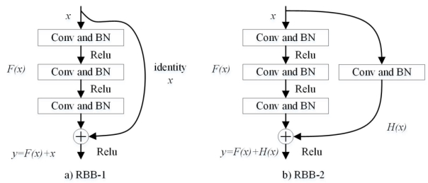
[37] | K. M. He, X. Y. Zhang, S. Q. Ren, Ren SQ, J. Sun, Deep residual learning for image recognition. Proceedings of the IEEE Conference on Computer Vision and Pattern Recognition (CVPR), (2016), 770–778. |
[38] | T. W. Rauber, F. Assis Boldt and F. M. Varejão, Heterogeneous feature models and feature selection applied to bearing fault diagnosis. IEEE T. Ind. Electron., 62 (2015), 637–646. |
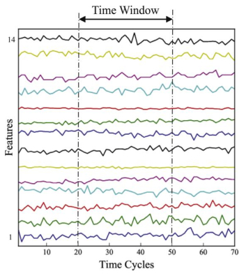
[39] | P. Lim, C. K. Goh and K. C. Tan, A time window neural network based framework for Remaining Useful Life estimation. 2016 International Joint Conference on Neural Networks (IJCNN), 1746–1753. |
[40] | Y. LeCun and Y. Bengio, Convolutional networks for images, speech, and time series, In: The handbook of brain theory and neural networks, MIT Press Cambridge, MA, USA, 1995. |
[41] | Y. Bengio, A. Courville and P. Vincent, Representation learning: A review and new perspectives. IEEE T. Pattern. Anal., 35 (2013), 1798–1828. |
[42] | M. Xiao, L. Wen, X. Li and L. Gao, Modeling of the feed-motor transient current in end milling by using varying-coefficient model. Math. Probl. Eng., 2015. |
[43] | T. Han, D. Jiang, Q. Zhao Q, L. Wang and K. Yin, Comparison of random forest, artificial neural networks and support vector machine for intelligent diagnosis of rotating machinery. Trans. I. Meas. Control., (2017), 1–13. |
[44] | PHM08 Challenge Data Set, NASA Data Repository, 2018. Available from: https://ti.arc.nasa.gov/tech/dash/groups/pcoe/prognostic-data-repository/#turbofan. |
[45] | S. Zheng, K. Ristovski, A. Farahat A and C. Gupta, Long short-term memory network for remaining useful life estimation. 2017 IEEE International Conference on Prognostics and Health Management (ICPHM), 88–95. |
[46] | S. K. Singh, S. Kumar, J. P. Dwivedi, A novel soft computing method for engine RUL prediction. Multimed. Tools Appl., (2017), 1–23. |
1. | Luca Biggio, Iason Kastanis, Prognostics and Health Management of Industrial Assets: Current Progress and Road Ahead, 2020, 3, 2624-8212, 10.3389/frai.2020.578613 | |
2. | Tarek Berghout, Leïla-Hayet Mouss, Ouahab Kadri, Lotfi Saïdi, Mohamed Benbouzid, Aircraft Engines Remaining Useful Life Prediction with an Improved Online Sequential Extreme Learning Machine, 2020, 10, 2076-3417, 1062, 10.3390/app10031062 | |
3. | Bin He, Long Liu, Dong Zhang, Digital Twin-Driven Remaining Useful Life Prediction for Gear Performance Degradation: A Review, 2021, 21, 1530-9827, 10.1115/1.4049537 | |
4. | Sergey Barkalov, Dmitry Dorofeev, Irina Fedorova, Alla Polovinkina, V. Breskich, S. Uvarova, Application of digital twins in the management of socio-economic systems, 2021, 244, 2267-1242, 11001, 10.1051/e3sconf/202124411001 | |
5. | Biao Wang, Yaguo Lei, Tao Yan, Naipeng Li, Liang Guo, Recurrent convolutional neural network: A new framework for remaining useful life prediction of machinery, 2020, 379, 09252312, 117, 10.1016/j.neucom.2019.10.064 | |
6. | Tarek Berghout, Leïla-Hayet Mouss, Toufik Bentrcia, Elhoussin Elbouchikhi, Mohamed Benbouzid, A deep supervised learning approach for condition-based maintenance of naval propulsion systems, 2021, 221, 00298018, 108525, 10.1016/j.oceaneng.2020.108525 | |
7. | Jinyang Jiao, Ming Zhao, Jing Lin, Kaixuan Liang, A comprehensive review on convolutional neural network in machine fault diagnosis, 2020, 417, 09252312, 36, 10.1016/j.neucom.2020.07.088 | |
8. | Xinyun Zhang, Yan Dong, Long Wen, Fang Lu, Wei Li, 2019, Remaining Useful Life Estimation Based on a New Convolutional and Recurrent Neural Network, 978-1-7281-0356-3, 317, 10.1109/COASE.2019.8843078 | |
9. | Liangwei Zhang, Jing Lin, Bin Liu, Zhicong Zhang, Xiaohui Yan, Muheng Wei, A Review on Deep Learning Applications in Prognostics and Health Management, 2019, 7, 2169-3536, 162415, 10.1109/ACCESS.2019.2950985 | |
10. | Zhao Zhang, Xinyu Li, Long Wen, Liang Gao, Yiping Gao, 2019, Fault Diagnosis Using Unsupervised Transfer Learning Based on Adversarial Network, 978-1-7281-0356-3, 305, 10.1109/COASE.2019.8842881 | |
11. | Ali Al-Dulaimi, Soheil Zabihi, Amir Asif, Arash Mohammed, NBLSTM: Noisy and Hybrid Convolutional Neural Network and BLSTM-Based Deep Architecture for Remaining Useful Life Estimation, 2020, 20, 1530-9827, 10.1115/1.4045491 | |
12. | Tao Li, YinQuan Yu, JinWen Yang, Long Zhang, WenBin Tu, Hao Yong, Method for Predicting Cutter Remaining Life Based on Multi-scale Cyclic Convolutional Network (MSRCNN), 2021, 1754, 1742-6588, 012218, 10.1088/1742-6596/1754/1/012218 | |
13. | Zhen Jia, Yaguang Luo, Dayang Wang, Quynh N. Dinh, Sophia Lin, Arnav Sharma, Ethan M. Block, Manyun Yang, Tingting Gu, Arne J. Pearlstein, Hengyong Yu, Boce Zhang, Nondestructive Multiplex Detection of Foodborne Pathogens with Background Microflora and Symbiosis Using a Paper Chromogenic Array and Advanced Neural Network, 2021, 09565663, 113209, 10.1016/j.bios.2021.113209 | |
14. | Jun Xia, Yunwen Feng, Cheng Lu, Chengwei Fei, Xiaofeng Xue, LSTM-based multi-layer self-attention method for remaining useful life estimation of mechanical systems, 2021, 125, 13506307, 105385, 10.1016/j.engfailanal.2021.105385 | |
15. | Seokgoo Kim, Nam Ho Kim, Joo-Ho Choi, A Study Toward Appropriate Architecture of System-Level Prognostics: Physics-Based and Data-Driven Approaches, 2021, 9, 2169-3536, 157960, 10.1109/ACCESS.2021.3129516 | |
16. | Angel J. Alfaro-Nango, Elias N. Escobar-Gomez, Eduardo Chandomi-Castellanos, Sabino Velazquez-Trujillo, Hector R. Hernandez-De-Leon, Lidya M. Blanco-Gonzalez, 2022, Predictive Maintenance Algorithm Based on Machine Learning for Industrial Asset, 978-1-6654-9607-0, 1489, 10.1109/CoDIT55151.2022.9803983 | |
17. | Amgad Muneer, Shakirah Mohd Taib, Suliman Mohamed Fati, Hitham Alhussian, Deep-Learning Based Prognosis Approach for Remaining Useful Life Prediction of Turbofan Engine, 2021, 13, 2073-8994, 1861, 10.3390/sym13101861 | |
18. | Seokgoo Kim, Joo-Ho Choi, Nam H. Kim, Challenges and Opportunities of System-Level Prognostics, 2021, 21, 1424-8220, 7655, 10.3390/s21227655 | |
19. | Manuel Arias Chao, Chetan Kulkarni, Kai Goebel, Olga Fink, Fusing physics-based and deep learning models for prognostics, 2022, 217, 09518320, 107961, 10.1016/j.ress.2021.107961 | |
20. | Viatcheslav P. Shuvalov, Boris P. Zelentsov, Irina G. Kvitkova, 2021, Optimization of Testing Intervals in the Conditions of Optical Fiber Periodic Predictive Control, 978-1-6654-3408-9, 346, 10.1109/APEIE52976.2021.9647546 | |
21. | Xianjun Du, Wenchao Jia, Ping Yu, Yaoke Shi, Bin Gong, RUL prediction based on GAM–CNN for rotating machinery, 2023, 45, 1678-5878, 10.1007/s40430-023-04062-8 | |
22. | Cheng Peng, Jiaqi Wu, Zhaohui Tang, Xinpan Yuan, Changyun Li, Tapan Senapati, A Spatio-Temporal Attention Mechanism Based Approach for Remaining Useful Life Prediction of Turbofan Engine, 2022, 2022, 1687-5273, 1, 10.1155/2022/9707940 | |
23. | Hongchun Sun, Chenchen Wu, Zunyang Lei, Uncertainty Measurement of the Prediction of the Remaining Useful Life of Rolling Bearings, 2022, 5, 2572-3901, 10.1115/1.4054392 | |
24. | Luca Biggio, Alexander Wieland, Manuel Arias Chao, Iason Kastanis, Olga Fink, Uncertainty-Aware Prognosis via Deep Gaussian Process, 2021, 9, 2169-3536, 123517, 10.1109/ACCESS.2021.3110049 | |
25. | Asefeh Asemi, Andrea Ko, Adeleh Asemi, Infoecology of the deep learning and smart manufacturing: thematic and concept interactions, 2022, 40, 0737-8831, 994, 10.1108/LHT-08-2021-0252 | |
26. | Narjes Davari, Bruno Veloso, Gustavo de Assis Costa, Pedro Mota Pereira, Rita P. Ribeiro, João Gama, A Survey on Data-Driven Predictive Maintenance for the Railway Industry, 2021, 21, 1424-8220, 5739, 10.3390/s21175739 | |
27. | Amgad Muneer, Shakirah Mohd Taib, Sheraz Naseer, Rao Faizan Ali, Izzatdin Abdul Aziz, Data-Driven Deep Learning-Based Attention Mechanism for Remaining Useful Life Prediction: Case Study Application to Turbofan Engine Analysis, 2021, 10, 2079-9292, 2453, 10.3390/electronics10202453 | |
28. | Jiachen Yao, Baochun Lu, Junli Zhang, Multi-Step-Ahead Tool State Monitoring Using Clustering Feature-Based Recurrent Fuzzy Neural Networks, 2021, 9, 2169-3536, 113443, 10.1109/ACCESS.2021.3104668 | |
29. | Mantas Landauskas, Loreta Saunoriene, Minvydas Ragulskis, 2021, Multiscale Diversity Index for RUL Analysis with Bernstein Polynomial Neural Networks, 9781450389839, 517, 10.1145/3459104.3459188 | |
30. | Xianli Liu, Shaoyang Liu, Xuebing Li, Bowen Zhang, Caixu Yue, Steven Y. Liang, Intelligent tool wear monitoring based on parallel residual and stacked bidirectional long short-term memory network, 2021, 60, 02786125, 608, 10.1016/j.jmsy.2021.06.006 | |
31. | Ibrahem M. A. Ibrahem, Ouassima Akhrif, Hany Moustapha, Martin Staniszewski, An Ensemble of Recurrent Neural Networks for Real Time Performance Modeling of Three-Spool Aero-Derivative Gas Turbine Engine, 2021, 143, 0742-4795, 10.1115/1.4051112 | |
32. | Jichao Zhuang, Minping Jia, Yifei Ding, Peng Ding, Temporal convolution-based transferable cross-domain adaptation approach for remaining useful life estimation under variable failure behaviors, 2021, 216, 09518320, 107946, 10.1016/j.ress.2021.107946 | |
33. | Khanh T. P. Nguyen, Kamal Medjaher, Do T. Tran, A review of artificial intelligence methods for engineering prognostics and health management with implementation guidelines, 2022, 0269-2821, 10.1007/s10462-022-10260-y | |
34. | Xuguo Yan, Xuhui Xia, Lei Wang, Zelin Zhang, A Cotraining-Based Semisupervised Approach for Remaining-Useful-Life Prediction of Bearings, 2022, 22, 1424-8220, 7766, 10.3390/s22207766 | |
35. | Amare Desalegn Fentaye, Valentina Zaccaria, Konstantinos Kyprianidis, Aircraft Engine Performance Monitoring and Diagnostics Based on Deep Convolutional Neural Networks, 2021, 9, 2075-1702, 337, 10.3390/machines9120337 | |
36. | Cheng Peng, Jiaqi Wu, Qilong Wang, Weihua Gui, Zhaohui Tang, Remaining Useful Life Prediction Using Dual-Channel LSTM with Time Feature and Its Difference, 2022, 24, 1099-4300, 1818, 10.3390/e24121818 | |
37. | Yuxin Wen, Md. Fashiar Rahman, Honglun Xu, Tzu-Liang Bill Tseng, Recent advances and trends of predictive maintenance from data-driven machine prognostics perspective, 2022, 187, 02632241, 110276, 10.1016/j.measurement.2021.110276 | |
38. | Kürşat İnce, Yakup Genc, Joint autoencoder-regressor deep neural network for remaining useful life prediction, 2023, 41, 22150986, 101409, 10.1016/j.jestch.2023.101409 | |
39. | Ye Zhu, Bo Xu, Zhenjie Luo, Zhiqiang Liu, Hao Wang, Chenglie Du, 2022, Prediction method of turbine engine RUL based on GA-SVR, 978-1-6654-5087-4, 1, 10.1109/AICIT55386.2022.9930303 | |
40. | Qiankun Hu, Yongping Zhao, Lihua Ren, Novel Transformer-based Fusion Models for Aero-engine Remaining Useful Life Estimation, 2023, 2169-3536, 1, 10.1109/ACCESS.2023.3277730 | |
41. | Suleyman Yildirim, Zeeshan A. Rana, Enhancing Aircraft Safety through Advanced Engine Health Monitoring with Long Short-Term Memory, 2024, 24, 1424-8220, 518, 10.3390/s24020518 | |
42. | Yucheng Wang, Min Wu, Xiaoli Li, Lihua Xie, Zhenghua Chen, Multivariate Time-Series Representation Learning via Hierarchical Correlation Pooling Boosted Graph Neural Network, 2024, 5, 2691-4581, 321, 10.1109/TAI.2023.3241896 | |
43. | Lin Song, Jun Wu, Liping Wang, Guo Chen, Yile Shi, Zhigui Liu, Remaining Useful Life Prediction of Rolling Bearings Based on Multi-Scale Attention Residual Network, 2023, 25, 1099-4300, 798, 10.3390/e25050798 | |
44. | Yasunari Matsuzaka, Yoshihiro Uesawa, Computational Models That Use a Quantitative Structure–Activity Relationship Approach Based on Deep Learning, 2023, 11, 2227-9717, 1296, 10.3390/pr11041296 | |
45. | Jun Guo, Dapeng Li, Baigang Du, A stacked ensemble method based on TCN and convolutional bi-directional GRU with multiple time windows for remaining useful life estimation, 2024, 150, 15684946, 111071, 10.1016/j.asoc.2023.111071 | |
46. | Gyeongho Kim, Jae Gyeong Choi, Sunghoon Lim, Using transformer and a reweighting technique to develop a remaining useful life estimation method for turbofan engines, 2024, 133, 09521976, 108475, 10.1016/j.engappai.2024.108475 | |
47. | Hairui Wang, Dongwen Li, Dongjun Li, Cuiqin Liu, Xiuqi Yang, Guifu Zhu, Remaining Useful Life Prediction of Aircraft Turbofan Engine Based on Random Forest Feature Selection and Multi-Layer Perceptron, 2023, 13, 2076-3417, 7186, 10.3390/app13127186 | |
48. | F Gougam, A Afia, MA Aitchikh, W Touzout, C Rahmoune, D Benazzouz, Computer numerical control machine tool wear monitoring through a data-driven approach, 2024, 16, 1687-8132, 10.1177/16878132241229314 | |
49. | Safa Ben Ayed, Roozbeh Sadeghian Broujeny, Rachid Tahar Hamza, Remaining Useful Life Prediction with Uncertainty Quantification Using Evidential Deep Learning, 2025, 15, 2449-6499, 37, 10.2478/jaiscr-2025-0003 | |
50. | Yucheng Wang, Min Wu, Ruibing Jin, Xiaoli Li, Lihua Xie, Zhenghua Chen, Local–Global Correlation Fusion-Based Graph Neural Network for Remaining Useful Life Prediction, 2025, 36, 2162-237X, 753, 10.1109/TNNLS.2023.3330487 | |
51. | Josue Luiz Dalboni da Rocha, Jesyin Lai, Pankaj Pandey, Phyu Sin M. Myat, Zachary Loschinskey, Asim K. Bag, Ranganatha Sitaram, Artificial Intelligence for Neuroimaging in Pediatric Cancer, 2025, 17, 2072-6694, 622, 10.3390/cancers17040622 | |
52. | Qian Zhao, Dian Zhang, Xiang Jia, Bo Guo, Fengchen Qian, 2024, Remaining Useful Life Prediction for Complex Systems by Fusing Multi-Level Information, 979-8-3503-5401-0, 1, 10.1109/PHM-Beijing63284.2024.10874767 | |
53. | Chengying Zhao, Jiajun Wang, Fengxia He, Xiaotian Bai, Huaitao Shi, Jialin Li, Xianzhen Huang, A fatigue life prediction method based on multi-signal fusion deep attention residual convolutional neural network, 2025, 235, 0003682X, 110646, 10.1016/j.apacoust.2025.110646 |
FDD001 | FDD002 | FDD003 | FDD004 | |
Engine units for training | 100 | 260 | 100 | 249 |
Engine units for testing | 100 | 259 | 100 | 248 |
Operating conditions | 1 | 6 | 1 | 6 |
Fault modes | 1 | 1 | 2 | 2 |
Numbers of RBB | 2 | 3 | 4 | 5 | 6 | ||
FD001 | RMSE | mean | 12.79 | 12.55 | 12.48 | 12.59 | 12.16 |
std | 0.2362 | 0.30 | 0.2003 | 0.3522 | 0.2253 | ||
Score | mean | 238.04 | 213.84 | 218.71 | 217.68 | 212.48 | |
std | 18.51 | 7.37 | 13.22 | 6.97 | 10.80 | ||
FD002 | RMSE | mean | 21.76 | 20.85 | 21.32 | 21.13 | 21.31 |
std | 1.4351 | 0.5931 | 0.8897 | 0.8085 | 0.3274 | ||
Score | mean | 2210.70 | 2087.77 | 2280.53 | 2308.74 | 2422.66 | |
std | 201.67 | 80.41 | 227.06 | 216.22 | 184.12 | ||
FD003 | RMSE | mean | 12.45 | 12.07 | 12.01 | 12.43 | 12.46 |
std | 0.4687 | 0.2060 | 0.2449 | 0.2532 | 0.2264 | ||
Score | mean | 185.18 | 177.42 | 180.76 | 191.75 | 194.87 | |
std | 13.95 | 4.53 | 6.96 | 5.20 | 6.73 | ||
FD004 | RMSE | mean | 24.97 | 25.45 | 27.56 | 28.31 | 28.56 |
std | 0.8341 | 1.0273 | 1.4200 | 0.8560 | 1.1873 | ||
Score | mean | 3400.44 | 3846.57 | 5463.13 | 6467.84 | 6750.94 | |
std | 246.84 | 529.68 | 733.53 | 1730.09 | 1972.85 |
MLP | SVM | DNN | LSTM | DCNN | DBN | MODBNE | Deep LSTM | Stacking Ensemble | Ensemble ResCNN | ||
FD001 | RMSE | 16.78 | 40.72 | 13.56 | 13.52 | 12.61 | 15.21 | 15.04 | 16.14 | 16.67 | 12.16 |
Score | 560.59 | 7703.33 | 348.3 | 431.7 | 273.7 | 417.59 | 334.23 | 338 | - | 212.48 | |
FD002 | RMSE | 28.78 | 52.99 | 24.61 | 24.42 | 22.36 | 27.12 | 25.05 | 24.49 | 25.57 | 20.85 |
Score | 14026.72 | 316483.31 | 15622 | 14459 | 10412 | 9031.64 | 5585.34 | 4450 | - | 2087.77 | |
FD003 | RMSE | 18.47 | 46.32 | 13.93 | 13.54 | 12.64 | 14.71 | 12.51 | 16.18 | 18.44 | 12.01 |
Score | 479.85 | 22541.58 | 364.3 | 347.3 | 284.1 | 442.43 | 421.91 | 852 | - | 180.76 | |
FD004 | RMSE | 30.96 | 59.96 | 24.31 | 24.21 | 23.31 | 29.88 | 28.66 | 28.17 | 26.76 | 24.97 |
Score | 10444.35 | 141122.19 | 16223 | 14322 | 12466 | 7954.51 | 6557.62 | 5550 | - | 3400.44 |
Numbers of RBB | 2 | 3 | 4 | 5 | 6 | |||||||
Prediction value | Increase (%) | Prediction value | Increase (%) | Prediction value | Increase (%) | Prediction value | Increase (%) | Prediction value | Increase (%) | |||
FD001 | RMSE | mean | 13.12 | 2.59 | 12.96 | 0.03 | 12.97 | 0.04 | 13.22 | 0.05 | 12.80 | 0.05 |
std | 0.46 | 96.49 | 0.54 | 0.82 | 0.48 | 1.41 | 0.70 | 0.98 | 0.69 | 2.04 | ||
Score | mean | 257.35 | 8.11 | 232.14 | 0.09 | 240.58 | 0.10 | 245.90 | 0.13 | 241.51 | 0.14 | |
std | 29.07 | 56.95 | 18.56 | 1.52 | 26.07 | 0.97 | 22.22 | 2.18 | 32.04 | 1.96 | ||
FD002 | RMSE | mean | 23.55 | 8.23 | 22.26 | 0.07 | 22.86 | 0.07 | 22.91 | 0.08 | 23.24 | 0.09 |
std | 6.09 | 324.64 | 4.51 | 6.61 | 4.43 | 3.98 | 4.04 | 4.00 | 2.00 | 5.10 | ||
Score | mean | 3872.75 | 75.18 | 3287.58 | 0.57 | 3853.95 | 0.69 | 4213.01 | 0.82 | 5098.84 | 1.10 | |
std | 4247.73 | 2006.28 | 3088.59 | 37.41 | 3117.10 | 12.73 | 3159.85 | 13.61 | 3149.85 | 16.11 | ||
FD003 | RMSE | mean | 12.83 | 3.05 | 12.39 | 0.03 | 12.38 | 0.03 | 12.88 | 0.04 | 13.05 | 0.05 |
std | 1.01 | 114.56 | 0.48 | 1.34 | 0.51 | 1.08 | 0.74 | 1.92 | 0.67 | 1.96 | ||
Score | mean | 211.77 | 14.36 | 189.66 | 0.07 | 194.98 | 0.08 | 209.71 | 0.09 | 221.64 | 0.14 | |
std | 55.90 | 300.51 | 11.99 | 1.64 | 14.06 | 1.02 | 21.19 | 3.07 | 27.39 | 3.07 | ||
FD004 | RMSE | mean | 26.40 | 5.71 | 27.35 | 0.07 | 30.72 | 0.11 | 31.80 | 0.12 | 32.54 | 0.14 |
std | 2.29 | 174.80 | 2.32 | 1.26 | 2.50 | 0.76 | 3.63 | 3.24 | 2.62 | 1.21 | ||
Score | mean | 5195.42 | 52.79 | 7167.56 | 0.86 | 17170.15 | 2.14 | 19357.47 | 1.99 | 24852.90 | 2.68 | |
std | 1190.74 | 382.39 | 2902.50 | 4.48 | 9314.31 | 11.70 | 8904.02 | 4.15 | 12696.79 | 5.44 |