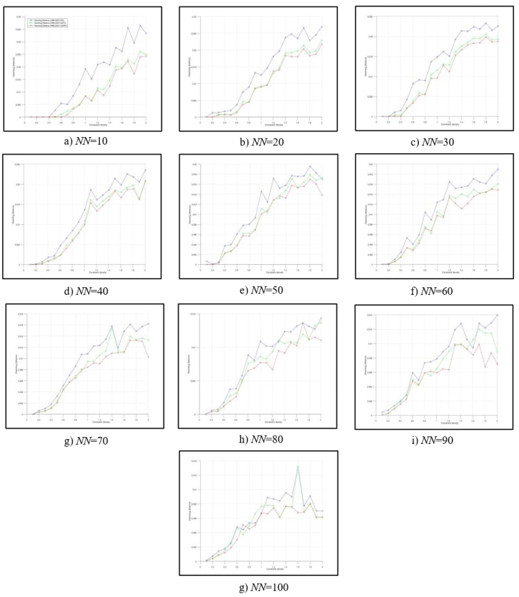
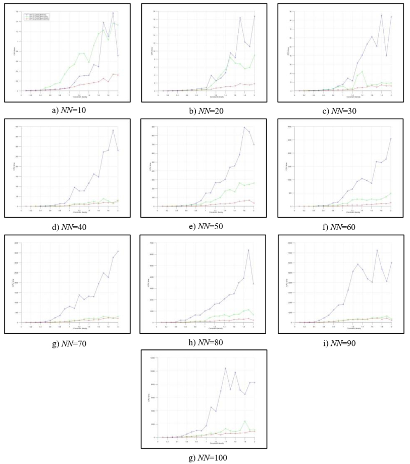
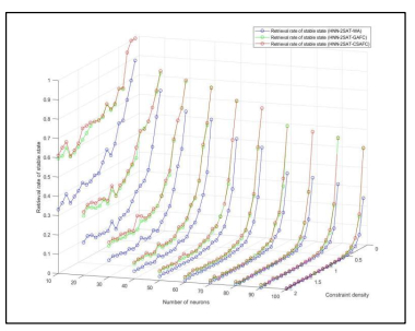
Within the swiftly evolving domain of neural networks, the discrete Hopfield-SAT model, endowed with logical rules and the ability to achieve global minima of SAT problems, has emerged as a novel prototype for SAT solvers, capturing significant scientific interest. However, this model shows substantial sensitivity to network size and logical complexity. As the number of neurons and logical complexity increase, the solution space rapidly contracts, leading to a marked decline in the model's problem-solving performance. This paper introduces a novel discrete Hopfield-SAT model, enhanced by Crow search-guided fuzzy clustering hybrid optimization, effectively addressing this challenge and significantly boosting solving speed. The proposed model unveils a significant insight: its uniquely designed cost function for initial assignments introduces a quantification mechanism that measures the degree of inconsistency within its logical rules. Utilizing this for clustering, the model utilizes a Crow search-guided fuzzy clustering hybrid optimization to filter potential solutions from initial assignments, substantially narrowing the search space and enhancing retrieval efficiency. Experiments were conducted with both simulated and real datasets for 2SAT problems. The results indicate that the proposed model significantly surpasses traditional discrete Hopfield-SAT models and those enhanced by genetic-guided fuzzy clustering optimization across key performance metrics: Global minima ratio, Hamming distance, CPU time, retrieval rate of stable state, and retrieval rate of global minima, particularly showing statistically significant improvements in solving speed. These advantages play a pivotal role in advancing the discrete Hopfield-SAT model towards becoming an exemplary SAT solver. Additionally, the model features exceptional parallel computing capabilities and possesses the potential to integrate with other logical rules. In the future, this optimized model holds promise as an effective tool for solving more complex SAT problems.
Citation: Caicai Feng, Saratha Sathasivam, Nurshazneem Roslan, Muraly Velavan. 2-SAT discrete Hopfield neural networks optimization via Crow search and fuzzy dynamical clustering approach[J]. AIMS Mathematics, 2024, 9(4): 9232-9266. doi: 10.3934/math.2024450
Within the swiftly evolving domain of neural networks, the discrete Hopfield-SAT model, endowed with logical rules and the ability to achieve global minima of SAT problems, has emerged as a novel prototype for SAT solvers, capturing significant scientific interest. However, this model shows substantial sensitivity to network size and logical complexity. As the number of neurons and logical complexity increase, the solution space rapidly contracts, leading to a marked decline in the model's problem-solving performance. This paper introduces a novel discrete Hopfield-SAT model, enhanced by Crow search-guided fuzzy clustering hybrid optimization, effectively addressing this challenge and significantly boosting solving speed. The proposed model unveils a significant insight: its uniquely designed cost function for initial assignments introduces a quantification mechanism that measures the degree of inconsistency within its logical rules. Utilizing this for clustering, the model utilizes a Crow search-guided fuzzy clustering hybrid optimization to filter potential solutions from initial assignments, substantially narrowing the search space and enhancing retrieval efficiency. Experiments were conducted with both simulated and real datasets for 2SAT problems. The results indicate that the proposed model significantly surpasses traditional discrete Hopfield-SAT models and those enhanced by genetic-guided fuzzy clustering optimization across key performance metrics: Global minima ratio, Hamming distance, CPU time, retrieval rate of stable state, and retrieval rate of global minima, particularly showing statistically significant improvements in solving speed. These advantages play a pivotal role in advancing the discrete Hopfield-SAT model towards becoming an exemplary SAT solver. Additionally, the model features exceptional parallel computing capabilities and possesses the potential to integrate with other logical rules. In the future, this optimized model holds promise as an effective tool for solving more complex SAT problems.

| [1] | S. A. Cook, The complexity of theorem-proving procedures, In: Logic, automata, and computational complexity: The works of Stephen A. Cook, 2023,143–152. https://doi.org/10.1145/3588287.3588297 |
| [2] |
J. J. Hopfield, Neural networks and physical systems with emergent collective computational abilities, P. Natl. Acad. Sci., 79 (1982), 2554–2558. https://doi.org/10.1073/pnas.79.8.2554 doi: 10.1073/pnas.79.8.2554

|
| [3] |
W. A. T. W. Abdullah, Logic programming on a neural network, Int. J. Intell. Syst., 7 (1992), 513–519. https://doi.org/10.1002/int.4550070604 doi: 10.1002/int.4550070604
|
| [4] |
S. Sathasivam, W. A. T. W. Abdullah, Logic mining in neural network: reverse analysis method, Computing, 91 (2011), 119–133. https://doi.org/10.1007/s00607-010-0117-9 doi: 10.1007/s00607-010-0117-9
|
| [5] | M. S. M. Kasihmuddin, M. A. Mansor, S. Sathasivam, Hybrid genetic algorithm in the Hopfield network for logic satisfiability problem, Pertanika J. Sci. Technol., 25 (2017), 139–152. |
| [6] |
S. Sathasivam, N. P. Fen, M. Velavan, Reverse analysis in higher order Hopfield network for higher order horn clauses, Appl. Math. Sci., 8 (2014), 601–612. https://doi.org/10.12988/ams.2014.310565 doi: 10.12988/ams.2014.310565
|
| [7] | M. A. Mansor, M. S. M. Kasihmuddin, S. Sathasivam, Artificial immune system paradigm in the Hopfield network for 3-satisfiability problem, Pertanika J. Sci. Technol., 25 (2017), 1173–1188. |
| [8] | M. S. M. Kasihmuddin, M. A. Mansor, S. Sathasivam, Discrete Hopfield neural network in restricted maximum k-satisfiability logic programming, Sains Malays., 47 (2018), 1327–1335. https://dx.doi.org/10.17576/jsm-2018-4706-30 |
| [9] |
S. Sathasivam, M. A. Mansor, A. I. M. Ismail, S. Z. M. Jamaludin, M. S. M. Kasihmuddin, M. Mamat, Novel random k satisfiability for k≤ 2 in Hopfield neural network, Sains Malays., 49 (2020), 2847–2857. https://doi.org/10.17576/jsm-2020-4911-23 doi: 10.17576/jsm-2020-4911-23
|
| [10] |
F. L. Azizan, S. Sathasivam, Randomised alpha-cut fuzzy logic hybrid model in Solving 3-satisfiability Hopfield neural network, Malays. J. Fundam. Appl. Sci., 19 (2023), 43–55. https://doi.org/10.11113/mjfas.v19n1.2697 doi: 10.11113/mjfas.v19n1.2697
|
| [11] |
S. A. Alzaeemi, S. Sathasivam, Examining the forecasting movement of palm oil price using RBFNN-2SATRA metaheuristic algorithms for logic mining, IEEE Access, 9 (2021), 22542–22557. https://doi.org/10.1109/ACCESS.2021.3054816 doi: 10.1109/ACCESS.2021.3054816
|
| [12] |
M. A. Mansor, M. S. M. Kasihmuddin, S. Sathasivam, VLSI circuit configuration using satisfiability logic in Hopfield network, Int. J. Intell. Syst. Appl., 8 (2016), 22. https://doi.org/10.5815/ijisa.2016.09.03 doi: 10.5815/ijisa.2016.09.03
|
| [13] |
M. A. Mansor, M. S. M. Kasihmuddin, S. Sathasivam, Enhanced Hopfield network for pattern satisfiability optimization, Int. J. Intell. Syst. Appl., 8 (2016), 27. https://doi.org/10.5815/ijisa.2016.11.04 doi: 10.5815/ijisa.2016.11.04
|
| [14] |
M. S. M. Kasihmuddin, M. A. Mansor, S. Sathasivam, Bezier curves satisfiability model in enhanced Hopfield network, Int. J. Intell. Syst. Appl., 8 (2016), 9. https://doi.org/10.5815/ijisa.2016.12.02 doi: 10.5815/ijisa.2016.12.02
|
| [15] |
M. S. M. Kasihmuddin, M. A. Mansor, S. Sathasivam, Students' performance via satisfiability reverse analysis method with Hopfield neural network, AIP Conf Proc., 2184 (2019), 060035. https://doi.org/10.1063/1.5136467 doi: 10.1063/1.5136467
|
| [16] |
L. C. Kho, M. S. M. Kasihmuddin, M. A. Mansor, S. Sathasivam, 2 Satisfiability logical rule by using ant colony optimization in Hopfield neural network, AIP Conf. Proc., 2184 (2019), 060009. https://doi.org/10.1063/1.5136441 doi: 10.1063/1.5136441
|
| [17] | M. A. Mansor, M. S. M. Kasihmuddin, S. Z. M. Jamaluddin, S. Sathasivam, Pattern 2 satisfiability snalysis via hybrid artificial bee colony algorithm as a learning algorithm, Commun. Comput. Appl. Math., 2 (2020), 12–18. |
| [18] |
S. Sathasivam, M. A. Mansor, M. S. M. Kasihmuddin, H. Abubakar, Election algorithm for random k satisfiability in the Hopfield neural network, Processes, 8 (2020), 568. https://doi.org/10.3390/pr8050568 doi: 10.3390/pr8050568
|
| [19] |
M. A. Mansor, M. S. M. Kasihmuddin, S. Sathasivam, Grey wolf optimization algorithm with discrete Hopfield neural network for 3 Satisfiability analysis, J. Phys.: Conf. Ser., 1821 (2021), 012038. https://doi.org/10.1088/1742-6596/1821/1/012038 doi: 10.1088/1742-6596/1821/1/012038
|
| [20] |
F. L. Azizan, S. Sathasivam, M. K. M Ali, N. Roslan, C. Feng, Hybridised network of fuzzy logic and a genetic algorithm in solving 3-satisfiability Hopfield neural networks, Axioms, 12 (2023), 250. https://doi.org/10.3390/axioms12030250 doi: 10.3390/axioms12030250
|
| [21] |
M. S. Mohd Kasihmuddin, N. S. Abdul Halim, S. Z. Mohd Jamaludin, M. Mansor, A. Alway, N. E. Zamri, et al., Logic mining approach: Shoppers' purchasing data extraction via evolutionary algorithm, J. Inf. Commun. Technol., 22 (2023), 309–335. https://doi.org/10.32890/jict2023.22.3.1 doi: 10.32890/jict2023.22.3.1
|
| [22] | S. Sathasivam, Applying fuzzy logic in neuro symbolic integration, World Appl. Sci. J., 17 (2012), 79–86. |
| [23] |
B. Bollobás, C. Borgs, J. T. Chayes, J. H. Kim, D. B. Wilson, The scaling window of the 2-SAT transition, Random Struct. Algor., 18 (2001), 201–256. https://doi.org/10.1002/rsa.1006 doi: 10.1002/rsa.1006
|
| [24] | M. Fürer, S. P. Kasiviswanathan, Algorithms for counting 2-SAT solutions and colorings with applications, In: Algorithmic aspects in information and management, 2007. https://doi.org/10.1007/978-3-540-72870-2_5 |
| [25] | M. Formann, F. Wagner, A packing problem with applications to lettering of maps, In: Proceedings of the seventh annual symposium on computational geometry, 1991. |
| [26] |
S. Ramnath, Dynamic digraph connectivity hastens minimum sum-of-diameters clustering, SIAM J. Discrete Math., 18 (2004), 272–286. https://doi.org/10.1137/S0895480102396099 doi: 10.1137/S0895480102396099
|
| [27] |
R. Miyashiro, T. Matsui, A polynomial-time algorithm to find an equitable home-away assignment, Oper. Res. Lett., 33 (2005), 235–241. https://doi.org/10.1016/j.orl.2004.06.004 doi: 10.1016/j.orl.2004.06.004
|
| [28] |
K. J. Batenburg, W. A. Kosters, Solving Nonograms by combining relaxations, Pattern Recogn., 42 (2009), 1672–1683. https://doi.org/10.1016/j.patcog.2008.12.003 doi: 10.1016/j.patcog.2008.12.003
|
| [29] | S. Sathasivam, Clauses representation comparison in neuro-symbolic integration, Proceedings of the World Congress on Engineering, 2010. |
| [30] |
J. C. Dunn, A fuzzy relative of the ISODATA process and its use in detecting compact well-separated clusters, J. Cyb., 3 (1973), 32–57. https://doi.org/10.1080/01969727308546046 doi: 10.1080/01969727308546046
|
| [31] |
J. C. Bezdek, R. Ehrlich, W. Full, FCM: The fuzzy c-means clustering algorithm, Comput. Geosci., 10 (1984), 191–203. https://doi.org/10.1016/0098-3004(84)90020-7 doi: 10.1016/0098-3004(84)90020-7
|
| [32] |
A. Askarzadeh, A novel metaheuristic method for solving constrained engineering optimization problems: Crow search algorithm, Comput. Struct., 169 (2016), 1–12. https://doi.org/10.1016/j.compstruc.2016.03.001 doi: 10.1016/j.compstruc.2016.03.001
|
| [33] | A. Saha, A. Bhattacharya, P. Das, A. K. Chakraborty, Crow search algorithm for solving optimal power flow problem, In: 2017 Second International Conference on Electrical, Computer and Communication Technologies (ICECCT), 2017. https://doi.org/10.1109/ICECCT.2017.8118028 |
| [34] | A. Lenin Fred, S. N. Kumar, P. Padmanaban, B. Gulyas, H. Ajay Kumar, Fuzzy-Crow search optimization for medical image segmentation, In: Applications of hybrid metaheuristic algorithms for image processing, 2020. https://doi.org/10.1007/978-3-030-40977-7_18 |
| [35] |
P. Upadhyay, J. K. Chhabra, Kapur's entropy based optimal multilevel image segmentation using Crow search algorithm, Appl. Soft Comput., 97 (2020), 105522. https://doi.org/10.1016/j.asoc.2019.105522 doi: 10.1016/j.asoc.2019.105522
|
| [36] |
G. Y. Abdallh, Z. Y. Algamal, A QSAR classification model of skin sensitization potential based on improving binary Crow search algorithm, Electron. J. Appl. Stat., 13 (2020), 86–95. https://doi.org/10.1285/i20705948v13n1p86 doi: 10.1285/i20705948v13n1p86
|
| [37] |
S. Arora, H. Singh, M. Sharma, S. Sharma, P. Anand, A new hybrid algorithm based on grey wolf optimization and Crow search algorithm for unconstrained function optimization and feature selection, IEEE Access, 7 (2019), 26343–26361. https://doi.org/10.1109/ACCESS.2019.2897325 doi: 10.1109/ACCESS.2019.2897325
|
| [38] | F. Davoodkhani, S. Arabi Nowdeh, A. Y. Abdelaziz, S. Mansoori, S. Nasri, M. Alijani, A new hybrid method based on gray wolf optimizer-Crow search algorithm for maximum power point tracking of photovoltaic energy system, In: Modern maximum power point tracking techniques for photovoltaic energy systems, 2020. https://doi.org/10.1007/978-3-030-05578-3_16 |
| [39] | A. B. Pratiwi, A hybrid cat swarm optimization-Crow search algorithm for vehicle routing problem with time windows, In: 2017 2nd international conferences on information technology, information systems and electrical engineering (ICITISEE), 2017. https://doi.org/10.1109/ICITISEE.2017.8285529 |
| [40] |
H. M. Farh, A. M. Al-Shaalan, A. M. Eltamaly, A. A. Al-Shamma'A, A novel Crow search algorithm auto-drive PSO for optimal allocation and sizing of renewable distributed generation, IEEE Access, 8 (2020), 27807–27820. https://doi.org/10.1109/ACCESS.2020.2968462 doi: 10.1109/ACCESS.2020.2968462
|
| [41] |
K. Gaddala, P. S. Raju, Merging lion with Crow search algorithm for optimal location and sizing of UPQC in distribution network, J. Control Autom. Electr. Syst., 31 (2020), 377–392. https://doi.org/10.1007/s40313-020-00564-1 doi: 10.1007/s40313-020-00564-1
|
| [42] |
R. Ganeshan, P. Rodrigues, Crow-AFL: Crow based adaptive fractional lion optimization approach for the intrusion detection, Wireless Pers. Commun., 111 (2020), 2065–2089. https://doi.org/10.1007/s11277-019-06972-0 doi: 10.1007/s11277-019-06972-0
|
| [43] |
D. K. Shende, S. S. Sonavane, Crow Whale-ETR: Crow Whale optimization algorithm for energy and trust aware multicast routing in WSN for IoT applications, Wireless Netw., 26 (2020), 4011–4029. https://doi.org/10.1007/s11276-020-02299-y doi: 10.1007/s11276-020-02299-y
|
| [44] |
A. M. Anter, A. E. Hassenian, D. Oliva, An improved fast fuzzy c-means using Crow search optimization algorithm for crop identification in agricultural, Expert Syst. Appl., 118 (2019), 340–354. https://doi.org/10.1016/j.eswa.2018.10.009 doi: 10.1016/j.eswa.2018.10.009
|
| [45] |
A. M. Anter, M. Ali, Feature selection strategy based on hybrid Crow search optimization algorithm integrated with chaos theory and fuzzy c-means algorithm for medical diagnosis problems, Soft Comput., 24 (2020), 1565–1584. https://doi.org/10.1007/s00500-019-03988-3 doi: 10.1007/s00500-019-03988-3
|
| [46] | L. O. Hall, J. C. Bezdek, S. Boggavarpu, A. Bensaid, Genetic fuzzy clustering, In: Proceedings of the first international joint conference of the north American fuzzy information processing society biannual conference, 1994,411–415. https://doi.org/10.1109/IJCF.1994.375077 |
| [47] |
N. Siswanto, A. N. Adianto, H. A. Prawira, A. Rusdiansyah, A Crow search algorithm for aircraft maintenance check problem and continuous airworthiness maintenance program, JSMI, 3 (2019), 10115–10123. https://doi.org/10.30656/jsmi.v3i2.1794 doi: 10.30656/jsmi.v3i2.1794
|
| [48] |
D. Gupta, S. Sundaram, J. J. Rodrigues, A. Khanna, An improved fault detection Crow search algorithm for wireless sensor network, Int. J. Commun. Syst., 36 (2023), e4136. https://doi.org/10.1002/dac.4136 doi: 10.1002/dac.4136
|
| [49] |
J. Mandala, M. C. Rao, Privacy preservation of data using Crow search with adaptive awareness probability, J. Inf. Secur. Appl., 44 (2019), 157–169. https://doi.org/10.1016/j.jisa.2018.12.005 doi: 10.1016/j.jisa.2018.12.005
|
| [50] |
R. Dash, S. Samal, R. Dash, R. Rautray, An integrated TOPSIS Crow search based classifier ensemble: In application to stock index price movement prediction, Appl. Soft Comput., 85 (2019), 105784. https://doi.org/10.1016/j.asoc.2019.105784 doi: 10.1016/j.asoc.2019.105784
|
| [51] |
A. G. Hussien, M. Amin, M. Wang, G. Liang, A. Alsanad, A.Gumaei, et al., Crow search algorithm: Theory, recent advances, and applications, IEEE Access, 8 (2020), 173548–173565. https://doi.org/10.1109/ACCESS.2020.3024108 doi: 10.1109/ACCESS.2020.3024108
|
| [52] | J. H. Holland, Adaptation in natural and artificial systems: An introductory analysis with applications to biology, control, and artificial intelligence, MIT Press, 1992. |
| [53] |
M. Alata, M. Molhim, A. Ramini, Optimizing of fuzzy c-means clustering algorithm using GA, Int. J. Comput. Inf. Eng., 2 (2008), 670–675. https://doi.org/10.5281/zenodo.1081049 doi: 10.5281/zenodo.1081049
|
| [54] |
Y. Ding, X. Fu, Kernel-based fuzzy c-means clustering algorithm based on genetic algorithm, Neurocomputing, 188 (2016), 233–238. https://doi.org/10.1016/j.neucom.2015.01.106 doi: 10.1016/j.neucom.2015.01.106
|
| [55] |
X. Wang, H. Wang, Driving behavior clustering for hazardous material transportation based on genetic fuzzy C-means algorithm, IEEE Access, 8 (2020), 11289–11296. https://doi.org/10.1109/ACCESS.2020.2964648 doi: 10.1109/ACCESS.2020.2964648
|
| [56] |
X. Cui, E. C. Yan, Fuzzy c-means cluster analysis based on variable length string genetic algorithm for the grouping of rock discontinuity sets, KSCE J. Civ. Eng., 24 (2020), 3237–3246. https://doi.org/10.1007/s12205-020-2188-2 doi: 10.1007/s12205-020-2188-2
|
| [57] | S. Sathasivam, Upgrading logic programming in Hopfield network, Sains Malays., 39 (2010), 115–128. |
| [58] |
M. Velavan, Z. R. bin Yahya, M. N. bin Abdul Halif, S. Sathasivam, Mean field theory in doing logic programming using Hopfield network, Mod. Appl. Sci., 10 (2016), 154. https://doi.org/10.5539/mas.v10n1p154 doi: 10.5539/mas.v10n1p154
|
Figures(20) / Tables(14)

Caicai Feng, Saratha Sathasivam, Nurshazneem Roslan, Muraly Velavan. 2-SAT discrete Hopfield neural networks optimization via Crow search and fuzzy dynamical clustering approach[J]. AIMS Mathematics, 2024, 9(4): 9232-9266. doi: 10.3934/math.2024450


 DownLoad: