A new solitary wave solution of the fractional phenomena Bogoyavlenskii equation via Bäcklund transformation

Yousef Jawarneh; Humaira Yasmin; Ali M. Mahnashi; Yousef Jawarneh; Humaira Yasmin; Ali M. Mahnashi

doi:10.3934/math.20241678

AIMS Mathematics

2024, Volume 9, Issue 12: 35308-35325. doi: 10.3934/math.20241678

Previous Article Next Article

Research article Special Issues

A new solitary wave solution of the fractional phenomena Bogoyavlenskii equation via Bäcklund transformation

1.
Department of Mathematics, College of Science, University of Ha'il, Ha'il 2440, Saudi Arabia
2.
Department of Basic Sciences, General Administration of Preparatory Year, King Faisal University, P.O. Box 400, Al Ahsa 31982, Saudi Arabia
3.
Department of Mathematics and Statistics, College of Science, King Faisal University, P.O. Box 400, Al Ahsa 31982, Saudi Arabia
4.
Department of Mathematics, Faculty of Science, Jazan University, P.O. Box 2097, Jazan 45142, Kingdom of Saudi Arabia

Received: 20 September 2024 Revised: 04 December 2024 Accepted: 06 December 2024 Published: 18 December 2024
MSC : 34G20, 35A20, 35A22, 35R11

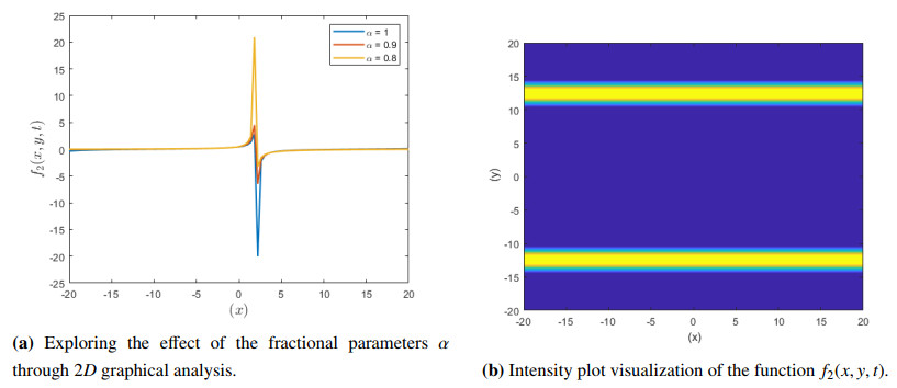
In this paper, we use the Riccati–Bernoulli sub-ODE method in conjunction with the Bäcklund transformation to find out the exact solutions of the nonlinear time–space fractional Bogoyavlenskii equation. The obtained solutions encompass multiple kink solitary wave solutions that are quite unique and important in addition to solutions presented in hyperbolic, trigonometric, and rational function forms. This equation describes central factors influencing its behavior including fluid dynamics in shallow water waves and plasma, which demonstrates our conclusions have broad applications for such systems. We also study the effect of the fractional order parameter ($ \alpha $) on solutions and plot their behavior using MATLAB in two dimensions. This work also contributes to the knowledge of the physical structures of the fractional Bogoyavlenskyi equation apart from showcasing the potential of the Riccati–Bernoulli sub-ODE method when applied to nonlinear fractional differential equations.
- fractional Bogoyavlenskii equation,
- Bäcklund transformation,
- non-linear differential equations,
- exact solutions
Citation: Yousef Jawarneh, Humaira Yasmin, Ali M. Mahnashi. A new solitary wave solution of the fractional phenomena Bogoyavlenskii equation via Bäcklund transformation[J]. AIMS Mathematics, 2024, 9(12): 35308-35325. doi: 10.3934/math.20241678

Related Papers:

Abstract

In this paper, we use the Riccati–Bernoulli sub-ODE method in conjunction with the Bäcklund transformation to find out the exact solutions of the nonlinear time–space fractional Bogoyavlenskii equation. The obtained solutions encompass multiple kink solitary wave solutions that are quite unique and important in addition to solutions presented in hyperbolic, trigonometric, and rational function forms. This equation describes central factors influencing its behavior including fluid dynamics in shallow water waves and plasma, which demonstrates our conclusions have broad applications for such systems. We also study the effect of the fractional order parameter ($ \alpha $) on solutions and plot their behavior using MATLAB in two dimensions. This work also contributes to the knowledge of the physical structures of the fractional Bogoyavlenskyi equation apart from showcasing the potential of the Riccati–Bernoulli sub-ODE method when applied to nonlinear fractional differential equations.

References

[1]	M. Almheidat, H. Yasmin, M. Al Huwayz, R. Shah, S. A. El-Tantawy, A novel investigation into time-fractional multi-dimensional Navier–Stokes equations within Aboodh transform, Open Phys., 22 (2024), 20240081. https://doi.org/10.1515/phys-2024-0081 doi: 10.1515/phys-2024-0081
[2]	M. M. Al-Sawalha, H. Yasmin, S. Muhammad, Y. Khan, R. Shah, Optimal power management of a stand-alone hybrid energy management system: hydro-photovoltaic-fuel cell, Ain Shams Eng. J., 15 (2024), 103089. https://doi.org/10.1016/j.asej.2024.103089 doi: 10.1016/j.asej.2024.103089
[3]	A. H. Ganie, H. Yasmin, A. A. Alderremy, A. S. Alshehry, S. Aly, Fractional view analytical analysis of generalized regularized long wave equation, Open Phys., 22 (2024), 20240025. https://doi.org/10.1515/phys-2024-0025 doi: 10.1515/phys-2024-0025
[4]	A. S. Alshehry, H. Yasmin, R. Shah, A. Ali, I. Khan, Fractional-order view analysis of Fisher's and foam drainage equations within Aboodh transform, Eng. Computation., 41 (2024), 489–515. https://doi.org/10.1108/EC-08-2023-0475 doi: 10.1108/EC-08-2023-0475
[5]	H. Yasmin, A. S. Alshehry, A. H. Ganie, A. M. Mahnashi, R. Shah, Perturbed Gerdjikov–Ivanov equation: soliton solutions via Backlund transformation, Optik, 298 (2024), 171576. https://doi.org/10.1016/j.ijleo.2023.171576 doi: 10.1016/j.ijleo.2023.171576
[6]	H. Durur, A. Yokus, ($1/G'$)-Açılım metodunu kullanarak Sawada–Kotera denkleminin hiperbolik yürüyen dalga cözümleri, (Turkish), Afyon Kocatepe Üniversitesi Fen Ve Mühendislik Bilimleri Dergisi, 19 (2019), 615–619. https://doi.org/10.35414/akufemubid.559048 doi: 10.35414/akufemubid.559048
[7]	Sirendaoreji, S. Jiong, Auxiliary equation method for solving nonlinear partial differential equations, Phys. Lett. A, 309 (2003), 387–396. https://doi.org/10.1016/S0375-9601(03)00196-8 doi: 10.1016/S0375-9601(03)00196-8
[8]	S. Abbasbandy, F. S. Zakaria, Soliton solutions for the fifth-order KdV equation with the homotopy analysis method, Nonlinear Dyn., 51 (2008), 83–87. https://doi.org/10.1007/s11071-006-9193-y doi: 10.1007/s11071-006-9193-y
[9]	A. Korkmaz, O. E. Hepson, K. Hosseini, H. Rezazadeh, M. Eslami, Sine-Gordon expansion method for exact solutions to conformable time fractional equations in RLW-class, J. King Saud Univ. Sci., 32 (2020), 567–574. https://doi.org/10.1016/j.jksus.2018.08.013 doi: 10.1016/j.jksus.2018.08.013
[10]	Z.-Y. Zhang, Exact traveling wave solutions of the perturbed Klein–Gordon equation with quadratic nonlinearity in (1+1)-dimension, Part Ⅰ: without local inductance and dissipation effect, Turk. J. Phys., 37 (2013), 259–267. https://doi.org/10.3906/fiz-1205-13 doi: 10.3906/fiz-1205-13
[11]	Z.-Y. Zhang, Z.-H. Liu, X.-J. Miao, Y.-Z. Chen, New exact solutions to the perturbed nonlinear Schrödinger's equation with Kerr law nonlinearity, Appl. Math. Comput., 216 (2010), 3064–3072. https://doi.org/10.1016/j.amc.2010.04.026 doi: 10.1016/j.amc.2010.04.026
[12]	Z.-Y. Zhang, Z.-H. Liu, X.-J. Miao, Y.-Z. Chen, Qualitative analysis and traveling wave solutions for the perturbed nonlinear Schrödinger's equation with Kerr law nonlinearity, Phys. Lett. A, 375 (2011), 1275–1280. https://doi.org/10.1016/j.physleta.2010.11.070 doi: 10.1016/j.physleta.2010.11.070
[13]	M. N. Khan, Siraj-ul-Islam, I. Hussain, I. Ahmad, H. Ahmad, A local meshless method for the numerical solution of space-dependent inverse heat problems, Math. Method. Appl. Sci., 44 (2021), 3066–3079. https://doi.org/10.1002/mma.6439 doi: 10.1002/mma.6439
[14]	M. N. Khan, I. Ahmad, H. Ahmad, A radial basis function collocation method for space-dependent inverse heat problems, J. Appl. Comput. Mech., 6 (2020), 1187–1199. https://doi.org/10.22055/JACM.2020.32999.2123 doi: 10.22055/JACM.2020.32999.2123
[15]	K. R. Kamal, G. Rahmat, K. Shah, On the numerical approximation of three-dimensional time fractional convection-diffusion equations, Math. Probl. Eng., 2021 (2021), 4640467. https://doi.org/10.1155/2021/4640467 doi: 10.1155/2021/4640467
[16]	Y. Kai, Z. Yin, On the Gaussian traveling wave solution to a special kind of Schrödinger equation with logarithmic nonlinearity, Mod. Phys. Lett. B, 36 (2022), 2150543. https://doi.org/10.1142/S0217984921505436 doi: 10.1142/S0217984921505436
[17]	Y. Kai, Z. Yin, Linear structure and soliton molecules of Sharma-Tasso-Olver-Burgers equation, Phys. Lett. A, 452 (2022), 128430. https://doi.org/10.1016/j.physleta.2022.128430 doi: 10.1016/j.physleta.2022.128430
[18]	C. Zhu, S. A. Idris, M. E. M. Abdalla, S. Rezapour, S. Shateyi, B. Gunay, Analytical study of nonlinear models using a modified Schrödinger's equation and logarithmic transformation, Results Phys., 55 (2023), 107183. https://doi.org/10.1016/j.rinp.2023.107183 doi: 10.1016/j.rinp.2023.107183
[19]	T. A. A. Ali, Z. Xiao, H. Jiang, B. Li, A class of digital integrators based on trigonometric quadrature rules, IEEE Trans. Ind. Electron., 71 (2024), 6128–6138. https://doi.org/10.1109/TIE.2023.3290247 doi: 10.1109/TIE.2023.3290247
[20]	A. Zulfiqar, J. Ahmad, Soliton solutions of fractional modified unstable Schrödinger equation using Exp-function method, Results Phys., 19 (2020), 103476. https://doi.org/10.1016/j.rinp.2020.103476 doi: 10.1016/j.rinp.2020.103476
[21]	M. A. Akbar, N. H. M. Ali, M. T. Islam, Multiple closed form solutions to some fractional order nonlinear evolution equations in physics and plasma physics, AIMS Math., 4 (2019), 397–411. https://doi.org/10.3934/math.2019.3.397 doi: 10.3934/math.2019.3.397
[22]	T. Liu, Exact solutions to time-fractional fifth order KdV equation by trial equation method based on symmetry, Symmetry, 11 (2019), 742. https://doi.org/10.3390/sym11060742 doi: 10.3390/sym11060742
[23]	L. Bai, J. Qi, Y. Sun, Physical phenomena analysis of solution structures in a nonlinear electric transmission network with dissipative elements, Eur. Phys. J. Plus, 139 (2024), 9. https://doi.org/10.1140/epjp/s13360-023-04736-1 doi: 10.1140/epjp/s13360-023-04736-1
[24]	L. Bai, J. Qi, Y. Sun, Further physical study about solution structures for nonlinear q-deformed Sinh–Gordon equation along with bifurcation and chaotic behaviors, Nonlinear Dyn., 111 (2023), 20165–20199. https://doi.org/10.1007/s11071-023-08882-0 doi: 10.1007/s11071-023-08882-0
[25]	W. Chen, Time-space fabric underlying anomalous diffusion, Chaos Soliton. Fract., 28 (2006), 923–929. https://doi.org/10.1016/j.chaos.2005.08.199 doi: 10.1016/j.chaos.2005.08.199
[26]	W. Chen, F. Wang, B. Zheng, W. Cai, Non-Euclidean distance fundamental solution of Hausdorff derivative partial differential equations, Eng. Anal. Bound. Elem., 84 (2017), 213–219. https://doi.org/10.1016/j.enganabound.2017.09.003 doi: 10.1016/j.enganabound.2017.09.003
[27]	J.-H. He, A tutorial review on fractal spacetime and fractional calculus, Int. J. Theor. Phys., 53 (2014), 3698–3718. https://doi.org/10.1007/s10773-014-2123-8 doi: 10.1007/s10773-014-2123-8
[28]	J.-H. He, Seeing with a single scale is always unbelieving: from magic to two-scale fractal, Therm. Sci., 25 (2021), 1217–1219. https://doi.org/10.2298/TSCI2102217H doi: 10.2298/TSCI2102217H
[29]	M. Z. Sarikaya, H. Budak, F. Usta, On generalized the conformable fractional calculus, TWMS J. Appl. Eng. Math., 9 (2019), 792–799.
[30]	O. I. Bogoyavlenskii, Breaking solitons in 2+1-dimensional integrable equations, Russ. Math. Surv., 45 (1990), 1–86. https://doi.org/10.1070/RM1990v045n04ABEH002377 doi: 10.1070/RM1990v045n04ABEH002377
[31]	Y.-Z. Peng, M. Shen, On exact solutions of Bogoyavlenskii equation, Pramana J. Phys., 67 (2006), 449–456. https://doi.org/10.1007/s12043-006-0005-1 doi: 10.1007/s12043-006-0005-1
[32]	A. Malik, F. Chand, H. Kumar, S. C. Mishra, Exact solutions of the Bogoyavlenskii equation using the multiple $G'/G$-expansion method, Comput. Math. Appl., 64 (2012), 2850–2859. https://doi.org/10.1016/j.camwa.2012.04.018 doi: 10.1016/j.camwa.2012.04.018
[33]	E. H. M. Zahran, M. M. A. Khater, Modified extended tanh-function method and its applications to the Bogoyavlenskii equation, Appl. Math. Model., 40 (2016), 1769–1775. https://doi.org/10.1016/j.apm.2015.08.018 doi: 10.1016/j.apm.2015.08.018
[34]	M. N. Alam, C. Tunc, An analytical method for solving exact solutions of the nonlinear Bogoyavlenskii equation and the nonlinear diffusive predator-prey system, Alex. Eng. J., 55 (2016), 1855–1865. https://doi.org/10.1016/j.aej.2016.04.024 doi: 10.1016/j.aej.2016.04.024
[35]	A. S. Alshehry, H. Yasmin, M. A. Shah, R. Shah, Analyzing fuzzy fractional Degasperis–Procesi and Camassa–Holm equations with the Atangana–Baleanu operator, Open Phys., 22 (2024), 20230191. https://doi.org/10.1515/phys-2023-0191 doi: 10.1515/phys-2023-0191
[36]	A. S. Alshehry, H. Yasmin, A. A. Khammash, R. Shah, Numerical analysis of dengue transmission model using Caputo–Fabrizio fractional derivative, Open Phys., 22 (2024), 20230169. https://doi.org/10.1515/phys-2023-0169 doi: 10.1515/phys-2023-0169
[37]	A. S. Alshehry, A. M. Mahnashi, Analyzing fractional PDE system with the Caputo operator and Mohand transform techniques, AIMS Math., 9 (2024), 32157–32181. https://doi.org/10.3934/math.20241544 doi: 10.3934/math.20241544
[38]	H. Yasmin, A. H. Almuqrin, Efficient solutions for time fractional Sawada-Kotera, Ito, and Kaup-Kupershmidt equations using an analytical technique, AIMS Math., 9 (2024), 20441–20466. https://doi.org/10.3934/math.2024994 doi: 10.3934/math.2024994
[39]	H. Yasmin, A. H. Almuqrin, Analytical study of time-fractional heat, diffusion, and Burger's equations using Aboodh residual power series and transform iterative methodologies, AIMS Math., 9 (2024), 16721–16752. https://doi.org/10.3934/math.2024811 doi: 10.3934/math.2024811
[40]	M. A. E. Abdelrahman, M. A. Sohaly, Solitary waves for the modified Korteweg-de Vries equation in deterministic case and random case, J. Phys. Math., 8 (2017), 214. https://doi.org/10.4172/2090-0902.1000214 doi: 10.4172/2090-0902.1000214
[41]	M. A. E. Abdelrahman, M. A. Sohaly, Solitary waves for the nonlinear Schrödinger problem with the probability distribution function in the stochastic input case, Eur. Phys. J. Plus, 132 (2017), 339. https://doi.org/10.1140/epjp/i2017-11607-5 doi: 10.1140/epjp/i2017-11607-5
[42]	X.-F. Yang, Z.-C. Deng, Y. Wei, A Riccati-Bernoulli sub-ODE method for nonlinear partial differential equations and its application, Adv. Differ. Equ., 2015 (2015), 117.
[43]	D. Lu, Q. Shi, New Jacobi elliptic functions solutions for the combined KdV-mKdV equation, Internatinal Journal of Nonlinear Science, 10 (2010), 320–325.
[44]	Y. Zhang, Solving STO and KD equations with modified Riemann–Liouville derivative using improved ($G/G'$)-expansion function method, International Journal of Applied Mathematics, 45 (2015), 16–22.
[45]	J. Lu, S. Shen, L. Chen, Variational approach for time-space fractal Bogoyavlenskii equation, Alex. Eng. J., 97 (2024), 294–301. https://doi.org/10.1016/j.aej.2024.04.031 doi: 10.1016/j.aej.2024.04.031

Reader Comments

Your name:*

Email:*
© 2024 the Author(s), licensee AIMS Press. This is an open access article distributed under the terms of the Creative Commons Attribution License (http://creativecommons.org/licenses/by/4.0)