Stability analysis of a class of nonlinear magnetic diffusion equations and its fully implicit scheme

Gao Chang; Chunsheng Feng; Jianmeng He; Shi Shu; Gao Chang; Chunsheng Feng; Jianmeng He; Shi Shu

doi:10.3934/math.20241014

AIMS Mathematics

2024, Volume 9, Issue 8: 20843-20864. doi: 10.3934/math.20241014

Previous Article Next Article

Research article Special Issues

Stability analysis of a class of nonlinear magnetic diffusion equations and its fully implicit scheme

1.
School of Mathematics and Computational Science, Xiangtan University, Xiangtan, Hunan, 411105, China
2.
College of General Education, Shanxi Institute of Science and Technology, Jincheng, Shanxi, 048000, China

Received: 06 May 2024 Revised: 06 June 2024 Accepted: 13 June 2024 Published: 27 June 2024
MSC : 35L03, 35L65, 65M08

We studied a class of nonlinear magnetic diffusion problems with step-function resistivity $ \eta(e) $ in electromagnetically driven high-energy-density physics experiments. The stability of the nonlinear magnetic diffusion equation and its fully implicit scheme, based on the step-function resistivity approximation model $ \eta_\delta(e) $ with smoothing, were studied. A rigorous theoretical analysis was established for the approximate model of one-dimensional continuous equations using Gronwall's theorem. Following this, the stability of the fully implicit scheme was proved using bootstrapping and other methods. The correctness of the theoretical proof was verified through one-dimensional numerical experiments.
- nonlinear magnetic diffusion equation,
- step-function resistivity,
- stability,
- implicit finite volume method
Citation: Gao Chang, Chunsheng Feng, Jianmeng He, Shi Shu. Stability analysis of a class of nonlinear magnetic diffusion equations and its fully implicit scheme[J]. AIMS Mathematics, 2024, 9(8): 20843-20864. doi: 10.3934/math.20241014

Related Papers:

Abstract

We studied a class of nonlinear magnetic diffusion problems with step-function resistivity $ \eta(e) $ in electromagnetically driven high-energy-density physics experiments. The stability of the nonlinear magnetic diffusion equation and its fully implicit scheme, based on the step-function resistivity approximation model $ \eta_\delta(e) $ with smoothing, were studied. A rigorous theoretical analysis was established for the approximate model of one-dimensional continuous equations using Gronwall's theorem. Following this, the stability of the fully implicit scheme was proved using bootstrapping and other methods. The correctness of the theoretical proof was verified through one-dimensional numerical experiments.

References

[1]	C. Yan, B. Xiao, G. Wang, Y. Lu, P. Li, A finite volume scheme based on magnetic flux and electromagnetic energy flow for solving magnetic field diffusion problems, Chin. J. Comput. Phys., 39 (2021): 379–385. http://doi.org/10.19596/j.cnki.1001-246x.8430
[2]	C. Sun, Research on High Energy Density Physical Problems under Electromagnetic Loading (1), High Energ. Dens. Phys., 2 (2007): 82–92.
[3]	T. Burgess, Electrical resistivity model of metals, 4th International Conference on Megagauss Magnetic-Field Generation and Related Topics, 1986.
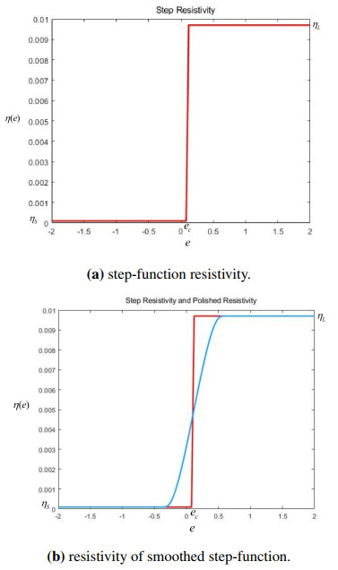
[4]	B. Xiao, G. Wang, An exact solution for the magnetic diffusion problem with a step-function resistivity model, Eur. Phys. J. Plus, 139 (2024), 305. http://doi.org/10.1140/epjp/s13360-024-05086-2 doi: 10.1140/epjp/s13360-024-05086-2
[5]	B. Xiao, Z. Gu, M. Kan, G. Wang, J. Zhao, Sharp-front wave of strong magnetic field diffusion in solid metal, Phys. Plasmas, 23 (2016), 082104. http://doi.org/10.1063/1.4960303 doi: 10.1063/1.4960303
[6]	C. Yan, B. Xiao, G. Wang, M. Kan, S. Duan, P. Li, et al., The second type of sharp-front wave mechanism of strong magnetic field diffusion in solid metal, AIP Adv., 9 (2019), 125008. http://doi.org/10.1063/1.5124436 doi: 10.1063/1.5124436
[7]	J. Hristov, Magnetic field diffusion in ferromagnetic materials: Fractional calculus approaches, IJOCTA, 11 (2021), 1–15. http://doi.org/10.11121/ijocta.01.2021.001100 doi: 10.11121/ijocta.01.2021.001100
[8]	O. Schnitzer, Fast penetration of megagauss fields into metallic conductors, Phys. Plasmas, 21 (2014), 082306. http://doi.org/10.1063/1.4892398 doi: 10.1063/1.4892398
[9]	Y. Zhou, L. Shen, G. Yuan, A Difference Method for Unconditional Stability and Convergence of Quasilinear Parabolic Systems with Parallelism Nature, Sci. China (Ser. A), 33 (2003), 310–324. http://doi.org/10.3969/j.issn.1674-7216.2003.04.003 doi: 10.3969/j.issn.1674-7216.2003.04.003
[10]	G. Yuan, Uniqueness and stability of difference solution with nonuniform meshes for nonlinear parabolic systems, Math. Numer. Sin., 22 (2000), 139–150.
[11]	G. Yuan, X. Hang, Conservative Parallel Schemes for Diffusion Equations, Chin. J. Comput. Phys., 27 (2010), 475–491.
[12]	G. Yuan, X. Hang, Adaptive combination algorithm of Picard and upwind-Newton (PUN) iteration for solving nonlinear diffusion equations, Sci. China (Ser. A), 2024, 1–16. https://www.sciengine.com/SSM/doi/10.1360/SSM-2023-0324
[13]	M. Bessemoulin-Chatard, F. Filbet, A Finite Volume Scheme for Nonlinear Degenerate Parabolic Equations, SIAM J. Sci. Comput., 34 (2012), B559–B583. http://doi.org/10.1137/110853807 doi: 10.1137/110853807
[14]	R. A. Adams, J. F. Fournier, Sobolev Spaces, New York: Academic Press, 2003.
[15]	Y. Chou, Applications of discrete functional analysis to the finite difference method, International Academic Publishers Pergamon Press, 1991.

Reader Comments

Your name:*

Email:*
© 2024 the Author(s), licensee AIMS Press. This is an open access article distributed under the terms of the Creative Commons Attribution License (http://creativecommons.org/licenses/by/4.0)