The single-valued neutrosophic hesitant fuzzy set (SV-NHFS) is a hybrid structure of the single-valued neutrosophic set and the hesitant fuzzy set that is designed for some incomplete, uncertain, and inconsistent situations in which each element has a few different values designed by the truth membership hesitant function, indeterminacy membership hesitant function, and falsity membership hesitant function. A strategic decision-making technique can help the decision-maker accomplish and analyze the information in an efficient manner. However, in our real lives, uncertainty will play a dominant role during the information collection phase. To handle such uncertainties in the data, we present a decision-making algorithm in the SV-NHFS environment. In this paper, we first presented the basic operational laws for SV-NHF information under Einstein's t-norm and t-conorm. Furthermore, important properties of Einstein operators, including the Einstein sum, product, and scalar multiplication, are done under SV-NHFSs. Then, we proposed a list of novel aggregation operators' names: Single-valued neutrosophic hesitant fuzzy Einstein weighted averaging, weighted geometric, order weighted averaging, and order weighted geometric aggregation operators. Finally, we discuss a multi-attribute decision-making (MADM) algorithm based on the proposed operators to address the problems in the SV-NHF environment. A numerical example is given to illustrate the work and compare the results with the results of the existing studies. Also, the sensitivity analysis and advantages of the stated algorithm are given in the work to verify and strengthen the study.
Citation: Muhammad Kamran, Shahzaib Ashraf, Nadeem Salamat, Muhammad Naeem, Thongchai Botmart. Cyber security control selection based decision support algorithm under single valued neutrosophic hesitant fuzzy Einstein aggregation information[J]. AIMS Mathematics, 2023, 8(3): 5551-5573. doi: 10.3934/math.2023280
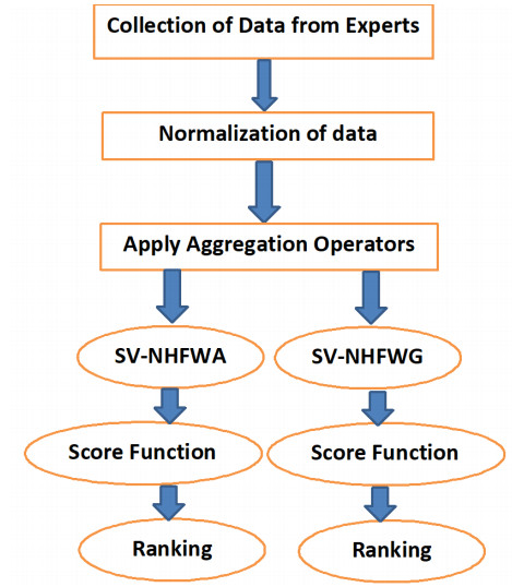
The single-valued neutrosophic hesitant fuzzy set (SV-NHFS) is a hybrid structure of the single-valued neutrosophic set and the hesitant fuzzy set that is designed for some incomplete, uncertain, and inconsistent situations in which each element has a few different values designed by the truth membership hesitant function, indeterminacy membership hesitant function, and falsity membership hesitant function. A strategic decision-making technique can help the decision-maker accomplish and analyze the information in an efficient manner. However, in our real lives, uncertainty will play a dominant role during the information collection phase. To handle such uncertainties in the data, we present a decision-making algorithm in the SV-NHFS environment. In this paper, we first presented the basic operational laws for SV-NHF information under Einstein's t-norm and t-conorm. Furthermore, important properties of Einstein operators, including the Einstein sum, product, and scalar multiplication, are done under SV-NHFSs. Then, we proposed a list of novel aggregation operators' names: Single-valued neutrosophic hesitant fuzzy Einstein weighted averaging, weighted geometric, order weighted averaging, and order weighted geometric aggregation operators. Finally, we discuss a multi-attribute decision-making (MADM) algorithm based on the proposed operators to address the problems in the SV-NHF environment. A numerical example is given to illustrate the work and compare the results with the results of the existing studies. Also, the sensitivity analysis and advantages of the stated algorithm are given in the work to verify and strengthen the study.

| [1] | C. A. Bana e Costa, P. Vincke, Multiple criteria decision aid: An overview, Readings in multiple criteria decision aid, Springer, Berlin, Heidelberg, 1990, 3–14. |
| [2] |
L. A. Zadeh, Fuzzy sets, Inf. Control., 8 (1965), 338–353. https://doi.org/10.1016/S0019-9958(65)90241-X doi: 10.1016/S0019-9958(65)90241-X

|
| [3] | K. T. Atanassov, Intuitionistic fuzzy sets, In Intuitionistic fuzzy sets, Physica, Heidelberg, 1999. |
| [4] |
G. Qian, H. Wang, X. Feng, Generalized hesitant fuzzy sets and their application in decision support system, Knowl.-Based Syst., 37 (2013), 357–365. https://doi.org/10.1016/j.knosys.2012.08.019 doi: 10.1016/j.knosys.2012.08.019
|
| [5] |
V. Torra, Hesitant fuzzy sets, Int. J. Intell. Syst., 25 (2010), 529–539. https://doi.org/10.1002/int.20418 doi: 10.1002/int.20418
|
| [6] |
R. M. Rodriguez, L. Martinez, F. Herrera, Hesitant fuzzy linguistic term sets for decision making, IEEE T. Fuzzy Syst., 20 (2011), 109–119. https://doi.org/10.1109/TFUZZ.2011.2170076 doi: 10.1109/TFUZZ.2011.2170076
|
| [7] | V. Torra, Y. Narukawa, On hesitant fuzzy sets and decision, In 2009 IEEE International Conference on Fuzzy Systems, IEEE, 2009, 1378–1382. https://doi.org/10.1109/FUZZY.2009.5276884 |
| [8] |
S. Faizi, T. Rashid, W. Sałabun, S. Zafar, J. Wkatró bski, Decision making with uncertainty using hesitant fuzzy sets, Int. J. Fuzzy Syst., 20 (2018), 93–103. https://doi.org/10.1007/s40815-017-0313-2 doi: 10.1007/s40815-017-0313-2
|
| [9] |
N. Chen, Z. Xu, M. Xia, Interval-valued hesitant preference relations and their applications to group decision making, Knowl. Based Syst., 37 (2013), 528–540. https://doi.org/10.1016/j.knosys.2012.09.009 doi: 10.1016/j.knosys.2012.09.009
|
| [10] |
G. Wei, X. Zhao, R. Lin, Some hesitant interval-valued fuzzy aggregation operators and their applications to multiple attribute decision making, Knowl. Based Syst., 46 (2013), 43–53. https://doi.org/10.1016/j.knosys.2013.03.004 doi: 10.1016/j.knosys.2013.03.004
|
| [11] |
S. Ashraf, S. Abdullah, T. Mahmood, F. Ghani, T. Mahmood, Spherical fuzzy sets and their applications in multi-attribute decision making problems, J. Intell. Fuzzy Syst., 36 (2019), 2829–2844. https://doi.org/10.3233/JIFS-172009 doi: 10.3233/JIFS-172009
|
| [12] |
R. R. Yager, Pythagorean membership grades in multicriteria decision making, IEEE T. Fuzzy Syst., 22 (2013), 958–965. https://doi.org/10.1109/TFUZZ.2013.2278989 doi: 10.1109/TFUZZ.2013.2278989
|
| [13] |
L. Wang, M. Ni, Z. Yu, L. Zhu, Power geometric operators of hesitant multiplicative fuzzy numbers and their application to multiple attribute group decision making, Math. Probl. Eng., 2014 (2014), 186502. https://doi.org/10.1155/2014/186502 doi: 10.1155/2014/186502
|
| [14] |
R. M. Rodríguez, L. Martínez, F. Herrera, Hesitant fuzzy linguistic term sets for decision-making, IEEE T. Fuzzy Syst., 20 (2012), 109–119. https://doi.org/10.1109/TFUZZ.2011.2170076 doi: 10.1109/TFUZZ.2011.2170076
|
| [15] |
Z. M. Zhang, C. Wu, Hesitant fuzzy linguistic aggregation operators and their applications to multiple attribute group decision-making, J. Intell. Fuzzy Syst., 26 (2014), 2185–2202. https://doi.org/10.3233/IFS-130893 doi: 10.3233/IFS-130893
|
| [16] |
J. Ye, Correlation coefficient of dual hesitant fuzzy sets and its application to multiple attribute decision making, Appl. Math. Model., 38 (2014), 659–666. https://doi.org/10.1016/j.apm.2013.07.010 doi: 10.1016/j.apm.2013.07.010
|
| [17] |
B. Zhu, Z. Xu, M. Xia, Dual hesitant fuzzy sets, J. Appl. Math., 2012 (2012). https://doi.org/10.1155/2012/879629 doi: 10.1155/2012/879629
|
| [18] |
G. Qian, H. Wang, X. Feng, Generalized hesitant fuzzy sets and their application in decision support system, Knowl.-Based Syst., 37 (2013), 357–365. https://doi.org/10.1016/j.knosys.2012.08.019 doi: 10.1016/j.knosys.2012.08.019
|
| [19] | J. Liu, M. Sun, Generalized power average operator of hesitant fuzzy numbers and its application in multiple attribute decision making, J. Comput. Inform. Syst., 9 (2013), 3051–3058. |
| [20] |
M. Xia, Z. Xu, Hesitant fuzzy information aggregation in decision making, Int. J. Approx. Reason., 52 (2011), 395–407. https://doi.org/10.1016/j.ijar.2010.09.002 doi: 10.1016/j.ijar.2010.09.002
|
| [21] |
Z. Xu, X. Zhang, Hesitant fuzzy multi-attribute decision making based on TOPSIS with incomplete weight information, Knowl.-Based Syst., 52 (2013), 53–64. https://doi.org/10.1016/j.knosys.2013.05.011 doi: 10.1016/j.knosys.2013.05.011
|
| [22] | D. Yu, Y. Wu, W. Zhou, Multi-criteria decision making based on Choquet integral under hesitant fuzzy environment, J. Comput. Inform. Syst., 7 (2011), 4506–4513. |
| [23] | F. Smarandache, A unifying field in logics, Neutrosophy: Neutrosophic probability, set and logic, 2005. |
| [24] |
J. Ye, A multicriteria decision-making method using aggregation operators for simplified neutrosophic sets, J. Intell. Fuzzy Syst., 26 (2014), 2459–2466. https://doi.org/10.3233/IFS-130916 doi: 10.3233/IFS-130916
|
| [25] |
J. Ye, Multiple-attribute decision-making method under a single-valued neutrosophic hesitant fuzzy environment, J. Intell. Syst., 24 (2015), 23–36. https://doi.org/10.1515/jisys-2014-0001 doi: 10.1515/jisys-2014-0001
|
| [26] | B. Farhadinia, Neutrosophic hesitant fuzzy set, In Hesitant Fuzzy Set, Springer, Singapore, 2021, 55–62. |
| [27] |
S. Ashraf, S. Abdullah, F. Smarandache, N. U. Amin, Logarithmic hybrid aggregation operators based on single valued neutrosophic sets and their applications in decision support systems, Symmetry, 11 (2019), 364. https://doi.org/10.3390/sym11030364 doi: 10.3390/sym11030364
|
| [28] |
D. Ripley, Paraconsistent logic, J. Philos. Logic, 44 (2015), 771–780. https://doi.org/10.1007/s10992-015-9358-6 doi: 10.1007/s10992-015-9358-6
|
| [29] |
F. Smarandache, Neutrosophic set–-a generalization of the intuitionistic fuzzy set, J. Def. Resour. Manag., 1 (2010), 107–116. https://doi.org/10.1109/GRC.2006.1635754 doi: 10.1109/GRC.2006.1635754
|
| [30] | H. Wang, F. Smarandache, Y. Zhang, R. Sunderraman, Single valued neutrosophic sets, Infinite Study, 2010. |
| [31] |
H. Kamacı, Linguistic single-valued neutrosophic soft sets with applications in game theory, Int. J. Intell. Syst., 36 (2021), 3917–3960. https://doi.org/10.1002/int.22445 doi: 10.1002/int.22445
|
| [32] |
R. P. Tan, W. D. Zhang, Decision-making method based on new entropy and refined single-valued neutrosophic sets and its application in typhoon disaster assessment, Appl. Intell., 51 (2021), 283–307. https://doi.org/10.1007/s10489-020-01706-3 doi: 10.1007/s10489-020-01706-3
|
| [33] |
C. Jana, M. Pal, Multi-criteria decision making process based on some single-valued neutrosophic Dombi power aggregation operators, Soft Comput., 25 (2021), 5055–5072. https://doi.org/10.1007/s00500-020-05509-z doi: 10.1007/s00500-020-05509-z
|
| [34] |
O. A. Razzaq, M. Fahad, N. A. Khan, Different variants of pandemic and prevention strategies: A prioritizing framework in fuzzy environment, Results Phys., 28 (2021), 104564. https://doi.org/10.1016/j.rinp.2021.104564 doi: 10.1016/j.rinp.2021.104564
|
| [35] |
P. Rani, J. Ali, R. Krishankumar, A. R. Mishra, F. Cavallaro, K. S. Ravichandran, An integrated single-valued neutrosophic combined compromise solution methodology for renewable energy resource selection problem, Energies, 14 (2021), 4594. https://doi.org/10.3390/en14154594 doi: 10.3390/en14154594
|
| [36] |
S. Ashraf, S. Abdullah, S. Zeng, H. Jin, F. Ghani, Fuzzy decision support modeling for hydrogen power plant selection based on single valued neutrosophic sine trigonometric aggregation operators, Symmetry, 12 (2020), 298. https://doi.org/10.3390/sym12020298 doi: 10.3390/sym12020298
|
| [37] | S. Ashraf, S. Abdullah, Decision support modeling for agriculture land selection based on sine trigonometric single valued neutrosophic information, Int. J. Neutros. Sci., 9 (2020), 60–73. |
| [38] |
H. Kamacı, H. Garg, S. Petchimuthu, Bipolar trapezoidal neutrosophic sets and their Dombi operators with applications in multicriteria decision making, Soft Comput., 25 (2021), 8417–8440. https://doi.org/10.1007/s00500-021-05768-4 doi: 10.1007/s00500-021-05768-4
|
| [39] |
H. Kamacı, S. Petchimuthu, E. Akçetin, Dynamic aggregation operators and Einstein operations based on interval-valued picture hesitant fuzzy information and their applications in multi-period decision making, Comput. Appl. Math., 40 (2021), 1–52. https://doi.org/10.1007/s40314-021-01510-w doi: 10.1007/s40314-021-01510-w
|
| [40] |
R. M. Zulqarnain, X. L. Xin, M. Saqlain, W. A. Khan, TOPSIS method based on the correlation coefficient of interval-valued intuitionistic fuzzy soft sets and aggregation operators with their application in decision-making, J. Math., 2021 (2021). https://doi.org/10.1155/2021/6656858 doi: 10.1155/2021/6656858
|
| [41] |
S. Naz, M. Akram, A. B. Saeid, A. Saadat, Models for MAGDM with dual hesitant q-rung orthopair fuzzy 2-tuple linguistic MSM operators and their application to COVID-19 pandemic, Expert Systems, 39 (2022), e13005. https://doi.org/10.1111/exsy.13005 doi: 10.1111/exsy.13005
|
Figures(1) / Tables(3)

Muhammad Kamran, Shahzaib Ashraf, Nadeem Salamat, Muhammad Naeem, Thongchai Botmart. Cyber security control selection based decision support algorithm under single valued neutrosophic hesitant fuzzy Einstein aggregation information[J]. AIMS Mathematics, 2023, 8(3): 5551-5573. doi: 10.3934/math.2023280


 DownLoad: