The unit generalized log Burr XII distribution: properties and application

Fiaz Ahmad Bhatti; Azeem Ali; G. G. Hamedani; Mustafa Ç. Korkmaz; Munir Ahmad; Fiaz Ahmad Bhatti; Azeem Ali; G. G. Hamedani; Mustafa Ç. Korkmaz; Munir Ahmad

doi:10.3934/math.2021592

AIMS Mathematics

2021, Volume 6, Issue 9: 10222-10252. doi: 10.3934/math.2021592

Previous Article Next Article

Research article

The unit generalized log Burr XII distribution: properties and application

1.
National College of Business Administration and Economics, Lahore Pakistan
2.
University of Veterinary and Animal Sciences, Lahore, Pakistan
3.
Marquette University, Milwaukee, WI 53201-1881, USA
4.
Artvin Çoruh University, Department of Measurement and Evaluation, Artvin, Turkey

Received: 31 December 2020 Accepted: 16 June 2021 Published: 12 July 2021
MSC : 60E05, 62E15, 62F10

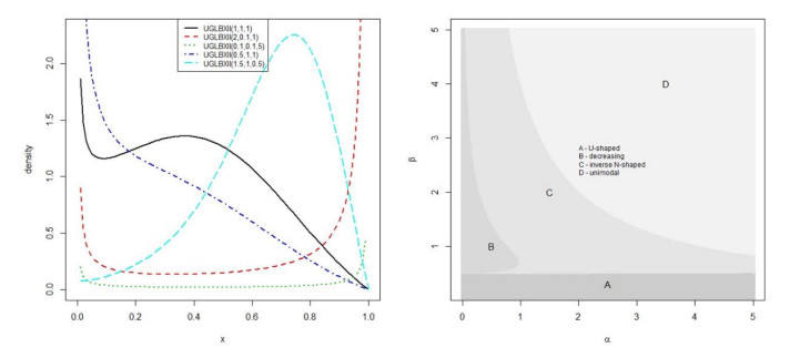
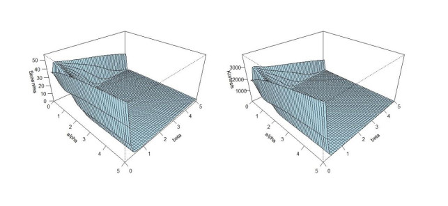
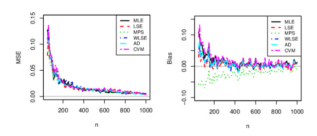
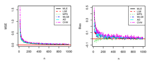
In this paper, a three-parameter bounded unit distribution with a flexible hazard rate called the unit generalized log Burr XII (UGLBXII) distribution is derived. To show the importance of the proposed distribution, we establish some of its mathematical properties such as random number generator, ordinary moments, generalized TL moments, conditional moments, reliability and uncertainty measures. We characterize the UGLBXII distribution via innovative techniques. We also present the bivariate‐ and multivariate‐type distributions via Morgenstern (Mor) family and via Clayton family. Six estimation methods such as the maximum likelihood, maximum product spacings, least squares, weighted least squares, Cramer-von Mises and Anderson-Darling methods are adopted to estimate its unknown parameters. We perform simulation studies on the basis of the graphical results to see the performance of the above estimators. Two real data sets are considered to prove the empirical superiority of the proposed model.
- generalized TL moments,
- maximum likelihood estimation,
- Pearson differential equation
Citation: Fiaz Ahmad Bhatti, Azeem Ali, G. G. Hamedani, Mustafa Ç. Korkmaz, Munir Ahmad. The unit generalized log Burr XII distribution: properties and application[J]. AIMS Mathematics, 2021, 6(9): 10222-10252. doi: 10.3934/math.2021592

Related Papers:

Abstract

In this paper, a three-parameter bounded unit distribution with a flexible hazard rate called the unit generalized log Burr XII (UGLBXII) distribution is derived. To show the importance of the proposed distribution, we establish some of its mathematical properties such as random number generator, ordinary moments, generalized TL moments, conditional moments, reliability and uncertainty measures. We characterize the UGLBXII distribution via innovative techniques. We also present the bivariate‐ and multivariate‐type distributions via Morgenstern (Mor) family and via Clayton family. Six estimation methods such as the maximum likelihood, maximum product spacings, least squares, weighted least squares, Cramer-von Mises and Anderson-Darling methods are adopted to estimate its unknown parameters. We perform simulation studies on the basis of the graphical results to see the performance of the above estimators. Two real data sets are considered to prove the empirical superiority of the proposed model.

References

[1]	N. L. Johnson, Systems of frequency curves generated by methods of translation, Biometrika, 36 (1949), 149–176. doi: 10.1093/biomet/36.1-2.149
[2]	C. W. Topp, F. C. Leone, A family of J-shaped frequency functions, J. Am. Stat. Assoc., 50 (1955), 209–219.
[3]	A. Grassia, On a family of distributions with argument between 0 and 1 obtained by transformation of the Gamma distribution and derived compound distributions, Austral. J. Statist., 19 (1977), 108–114. doi: 10.1111/j.1467-842X.1977.tb01277.x
[4]	J. Mazucheli, A. F. B. Menezes, S. Dey, Improved maximum-likelihood estimators for the parameters of the unit-gamma distribution, Commun. Stat.-Theor. M., 47 (2018) 3767–3778.
[5]	P. Kumaraswamy, A generalized probability density function for double-bounded random processes, J. Hydrol., 46 (1980), 79–88. doi: 10.1016/0022-1694(80)90036-0
[6]	B. C. Arnold, R. A. Groeneveld, Some properties of the Arcsine distribution, J. Am. Stat. Assoc., 75 (1980), 173–175. doi: 10.1080/01621459.1980.10477449
[7]	A. F. B. Menezes, J. Mazucheli, S. Dey, The unit-logistic distribution: different methods of estimation, Pesquisa Operacional, 38 (2018), 555–578. doi: 10.1590/0101-7438.2018.038.03.0555
[8]	O. E. Barndorff-Nielsen, B. Jørgensen, Some parametric models on the simplex, J. Multivariate Anal., 39 (1991), 106–116. doi: 10.1016/0047-259X(91)90008-P
[9]	J. Mazucheli, A. F. B. Menezes, S. Dey, The unit-Birnbaum-Saunders distribution with applications, Chilean Journal of Statistics, 9 (2018), 47–57.
[10]	J. Mazucheli, A. F. B. Menezes, M. E. Ghitany, The unit-Weibull distribution and associated inference, J. Appl. Probab. Stat., 13 (2018), 1–22.
[11]	J. Mazucheli, A. F. Maringa, S. Dey, Unit-Gompertz distribution with applications, Statistica, 79 (2019), 25–43.
[12]	J. Mazucheli, A. F. B. Menezes, S. Chakraborty, On the one parameter unit-Lindley distribution and its associated regression model for proportion data, J. Appl. Stat., 46 (2019), 700–714. doi: 10.1080/02664763.2018.1511774
[13]	E. Altun, G. M. Cordeiro, The unit-improved second-degree Lindley distribution: inference and regression modeling, Computation. Stat., 35 (2020), 259–279. doi: 10.1007/s00180-019-00921-y
[14]	M. E. Ghitany, J. Mazucheli, A. F. B. Menezes, F. Alqallaf, The unit-inverse Gaussian distribution: A new alternative to two-parameter distributions on the unit interval, Commun. Stat.-Theor. M., 48 (2019), 3423–3438. doi: 10.1080/03610926.2018.1476717
[15]	M. Ç. Korkmaz, The unit generalized half normal distribution: A new bounded distribution with inference and application. U. P. B. Sci. Bull., Series A, 82 (2020), 133–140.
[16]	M. Ç. Korkmaz, A new heavy-tailed distribution defined on the bounded interval: the logit slash distribution and its application, J. Appl. Stat., 47 (2020), 2097–2119.
[17]	M. Ç. Korkmaz, C. Chesneau, Z. S. Korkmaz, On the arcsecant hyperbolic normal distribution. properties, quantile regression modeling and applications, Symmetry, 13 (2021), 117. doi: 10.3390/sym13010117
[18]	M. Ç. Korkmaz, C. Chesneau, Z. S. Korkmaz, Transmuted unit Rayleigh quantile regression model: alternative to beta and Kumaraswamy quantile regression models, U. P. B. Sci. Bull., Series A, 2021.
[19]	F. A. Bhatti, A. Ali, G. G. Hamedani, M. Ahmad, On generalized log burr XII distribution, PJSOR, 14 (2018), 615–643. doi: 10.18187/pjsor.v14i3.1700
[20]	E. A. Elamir, A. H. Seheult, Trimmed L-moments, Comput. Stat. Data An., 43 (2003), 299–314.
[21]	J. R. Hosking, L-moments: analysis and estimation of distributions using linear combinations of order statistics, J. R. Stat. Soc. B, 52 (1990), 105–124.
[22]	Q. J. Wang, LH moments for statistical analysis of extreme events, Water Resour. Res., 33 (1997), 2841–2848. doi: 10.1029/97WR02134
[23]	M. Bayazit, B. Onoz, LL-moments for estimating low for quantiles, Hydrolog. Sci. J., 47 (2002), 707–720. doi: 10.1080/02626660209492975
[24]	G. K. Bhattacharyya, R. A. Johnson, Estimation of reliability in a multicomponent stress-strength model, J. Am. Stat. Assoc., 69 (1974), 966–970. doi: 10.1080/01621459.1974.10480238
[25]	S. Kotz, C. D. Lai, M. Xie, On the effect of redundancy for systems with dependent components, IIE Trans, 35 (2003), 1103–1110. doi: 10.1080/714044440
[26]	C. Shannon, A mathematical theory of communication, Bell System Tech. J., 27 (1948), 379–423. doi: 10.1002/j.1538-7305.1948.tb01338.x
[27]	A. M. Awad, A. J. Alawneh, Application of entropy to a life-time model, IMA J. Math. Control Inform., 4 (1987), 143–147. doi: 10.1093/imamci/4.2.143
[28]	A. Rényi, On measures of entropy and information, In: Proceedings of the Fourth Berkeley Symposium on Mathematical Statistics and Probability, Volume 1: Contributions to the Theory of Statistics, The Regents of the University of California, 1961.
[29]	J. Havrda, F. S. Charvat, Quantification method of classification processes: concept of structural-entropy, Kybernetika, 3 (1967), 30–35.
[30]	C. Tsallis, Possible generalization of Boltzmann-Gibbs statistics, J. Stat. Phys., 52 (1988), 479–487. doi: 10.1007/BF01016429
[31]	A. A. Al-babtain, I. Elbatal, H. M. Yousof, A new flexible three-parameter model: properties, Clayton copula, and modeling real data, Symmetry, 12 (2020), 440. doi: 10.3390/sym12030440
[32]	W. A. Glänzel, Some consequences of a characterization theorem based on truncated moments, Statistics, 21 (1990), 613–618.
[33]	R. C. H. Cheng, N. A. K. Amin, Maximum product of spacings estimation with application to the lognormal distribution, 1979, Math Report 79-1.
[34]	R. C. H. Cheng, N. A. K. Amin, Estimating parameters in continuous univariate distributions with a shifted origin, J. R. Stat. Soc. B, 45 (1983), 394–403.
[35]	B. Ranneby, The maximum spacing method. An estimation method related to the maximum likelihood method, Scand. J. Stat., 11 (1984), 93–112.
[36]	T. W. Anderson, D. A. Darling, Asymptotic theory of certain goodness of fit criteria based on stochastic processes, Ann. Math. Statist., 23 (1952), 193–212. doi: 10.1214/aoms/1177729437
[37]	G. Chen, N. Balakrishnan, A general purpose approximate goodness-of-fit test, J. Qual. Technol., 27 (1995), 154–161. doi: 10.1080/00224065.1995.11979578
[38]	M. Nadar, A. Papadopoulos, F. Kızılaslan, Statistical analysis for Kumaraswamy's distribution based on record data, Stat. Pap., 54 (2013), 355–369. doi: 10.1007/s00362-012-0432-7
[39]	L.Wang, Inference for the Kumaraswamy distribution under k-record values, J. Comput. Appl. Math., 321 (2017), 246–260. doi: 10.1016/j.cam.2017.02.037
[40]	G. M. Cordeiro, R. B. dos Santos, The Beta power distribution, Braz. J. Probab. Stat., 26 (2012), 88–112.

Reader Comments

Your name:*

Email:*
© 2021 the Author(s), licensee AIMS Press. This is an open access article distributed under the terms of the Creative Commons Attribution License (http://creativecommons.org/licenses/by/4.0)