Numerical simulation of the fractal-fractional reaction diffusion equations with general nonlinear

Khaled M. Saad; Manal Alqhtani; Khaled M. Saad; Manal Alqhtani

doi:10.3934/math.2021225

AIMS Mathematics

2021, Volume 6, Issue 4: 3788-3804. doi: 10.3934/math.2021225

Previous Article Next Article

Research article

Numerical simulation of the fractal-fractional reaction diffusion equations with general nonlinear

Khaled M. Saad ^{1,2
,
,},
Manal Alqhtani ¹

1.
Department of Mathematics, College of Sciences and Arts, Najran University, Najran, Kingdom of Saudi Arabia
2.
Department of Mathematics, Faculty of Applied Science, Taiz University, Taiz, Yemen

Received: 10 October 2020 Accepted: 18 January 2021 Published: 27 January 2021
MSC : Primary 26A33, 34A08; Secondary 35A20, 35A22

In this paper a new approach to the use of kernel operators derived from fractional order differential equations is proposed. Three different types of kernels are used, power law, exponential decay and Mittag-Leffler kernels. The kernel's fractional order and fractal dimension are the key parameters for these operators. The main objective of this paper is to study the effect of the fractal-fractional derivative order and the order of the nonlinear term, $ 1 < q < 2 $, in the equation on the behavior of numerical solutions of fractal-fractional reaction diffusion equations (FFRDE). Iterative approximations to the solutions of these equations are constructed by applying the theory of fractional calculus with the help of Lagrange polynomial functions. In key parameter regimes, all these iterative solutions based on a power kernel, an exponential kernel and a generalized Mittag-Leffler kernel are very close. Hence, iterative solutions obtained using one of these kernels are compared with full numerical solutions of the FFRDE and excellent agreement is found. All numerical solutions in this paper were obtained using Mathematica.
Citation: Khaled M. Saad, Manal Alqhtani. Numerical simulation of the fractal-fractional reaction diffusion equations with general nonlinear[J]. AIMS Mathematics, 2021, 6(4): 3788-3804. doi: 10.3934/math.2021225

Related Papers:

Abstract

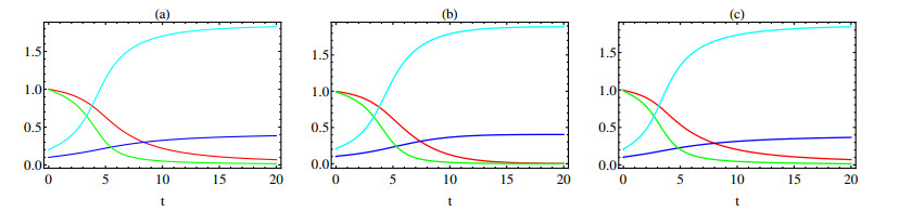
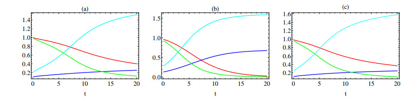
In this paper a new approach to the use of kernel operators derived from fractional order differential equations is proposed. Three different types of kernels are used, power law, exponential decay and Mittag-Leffler kernels. The kernel's fractional order and fractal dimension are the key parameters for these operators. The main objective of this paper is to study the effect of the fractal-fractional derivative order and the order of the nonlinear term, $ 1 < q < 2 $, in the equation on the behavior of numerical solutions of fractal-fractional reaction diffusion equations (FFRDE). Iterative approximations to the solutions of these equations are constructed by applying the theory of fractional calculus with the help of Lagrange polynomial functions. In key parameter regimes, all these iterative solutions based on a power kernel, an exponential kernel and a generalized Mittag-Leffler kernel are very close. Hence, iterative solutions obtained using one of these kernels are compared with full numerical solutions of the FFRDE and excellent agreement is found. All numerical solutions in this paper were obtained using Mathematica.

References

[1]	S. J. Liao, On the homotopy analysis method for nonlinear problems, Appl. Math. Comput., 147 (2004), 499-513.
[2]	K. M. Saad, E. H. AL-Shareef, M. S. Mohamed, X. J. Yang, Optimal q-homotopy analysis method for time-space fractional gas dynamics equation, Eur. Phys. J. Plus, 132 (2017), 23. doi: 10.1140/epjp/i2017-11303-6
[3]	K. M. Saad, A reliable analytical algorithm for spacetime fractional cubic isothermal autocatalytic chemical system, Pramana, 91 (2018), 51. doi: 10.1007/s12043-018-1620-3
[4]	K. M. Saad, E. H. F. AL-Shareef, A. K. Alomari, D. Baleanu, J. F. Gómez-Aguilar, On exact solutions for time-fractional Korteweg-de Vries and Korteweg-de Vries-Burgers equations using homotopy analysis transform method, Chinese J. Phys., 63 (2020), 149-162.
[5]	J. H. He, Variational iteration method-a kind of nonlinear analytical technique: some examples, Int. J. Non-Linear Mech., 34 (1999), 699-708. doi: 10.1016/S0020-7462(98)00048-1
[6]	K. M. Saad, E. H. F. Al-Sharif, Analytical study for time and time-space fractional Burgers equation, Adv. Differ. Equ., 2017 (2017), 300. doi: 10.1186/s13662-017-1358-0
[7]	X. C. Shi, L. L. Huang, Y. Zeng, Fast Adomian decomposition method for the Cauchy problem of the time-fractional reaction diffusion equation, Adv. Mech. Eng., 8 (2016), 1-5.
[8]	H. M. Srivastava, K. M. Saad, New approximate solution of the time-fractional Nagumo equation involving fractional integrals without singular kernel, Appl. Math. Inf. Sci., 14 (2020), 1-8. doi: 10.18576/amis/140101
[9]	H. M. Srivastava, K. M. Saad, E. H. F. Al-Sharif, A new analysis of the time-fractional and space-time fractional order Nagumo equation, J. Inf. Math. Sci., 10 (2018), 545-561.
[10]	A. Bueno-Orovio, D. Kay, K. Burrage, Fourier spectral methods for fractional-in-space reaction-diffusion equations, Bit. Numer. Math., 54 (2014), 937-954. doi: 10.1007/s10543-014-0484-2
[11]	Y. Takeuchi, Y. Yoshimoto, R. Suda, Second order accuracy finite difference methods for space-fractional partial differential equations, J. Comput. Appl. Math., 320 (2017), 101-119. doi: 10.1016/j.cam.2017.01.013
[12]	Y. K. Yildiray, K. Aydin, The solution of the Bagley Torvik equation with the generalized Taylor collocation method, J. Franklin Inst., 347 (2010), 452-466. doi: 10.1016/j.jfranklin.2009.10.007
[13]	M. M. Khader, K. M. Saad, A numerical approach for solving the fractional Fisher equation using Chebyshev spectral collocation method, Chaos Soliton. Fract., 110 (2018), 169-177. doi: 10.1016/j.chaos.2018.03.018
[14]	K. M. Saad, New fractional derivative with non-singular kernel for deriving Legendre spectral collocation method, Alex. Eng. J., 59 (2020), 1909-1917. doi: 10.1016/j.aej.2019.11.017
[15]	A. A. Kilbas, H. M. Srivastava, J. J. Trujillo, Theory and applications of fractional differential equations, Amsterdam: Elsevier (North-Holland) Science Publishers, 2006.
[16]	I. Podlubny, Fractional differential equations: An introduction to fractional derivatives, fractional differential equations, to methods of their solution and some of their applications, New York: Academic Press, 1999.
[17]	A. Atangana, Fractal-fractional differentiation and integration: connecting fractal calculus and fractional calculus to predict complex system, Chaos Soliton. Fract., 102 (2017), 396-406. doi: 10.1016/j.chaos.2017.04.027
[18]	M. Caputo, Linear models of dissipation whose Q is almost frequency independent: II, Geophys. J. Roy. Astron. Soc., 13 (1967), 529-539. doi: 10.1111/j.1365-246X.1967.tb02303.x
[19]	M. Caputo, M. Fabrizio, A new defnition of fractional derivative without singular kernel, Prog. Fract. Differ. Appl., 2 (2015), 73-85.
[20]	A. Atangana, D. Baleanu, New fractional derivative with nonlocal and non-singular kernel, Chaos Soliton. Fract., 20 (2016), 757-763.
[21]	Z. Li, Z. Liu, M. A. Khan, Fractional investigation of bank data with fractal-fractional Caputo derivative, Chaos Soliton. Fract., 131 (2020), 109528. doi: 10.1016/j.chaos.2019.109528
[22]	A. Atangana, M. A. Khan, Fatmawati, Modeling and analysis of competition model of bank data with fractal-fractional Caputo-Fabrizio operator, Alex. Eng. J., 59 (2020), 1985-1998. doi: 10.1016/j.aej.2019.12.032
[23]	W. Wanga, M. A. Khan, Analysis and numerical simulation of fractional model of bank data with fractal-fractional Atangana-Baleanu derivative, J. Comput. Appl. Math., 369 (2020), 112646. doi: 10.1016/j.cam.2019.112646
[24]	A. Atangana, A. Akgu, K. M. Owolabi, Analysis of fractal-fractional differential equations, Alex. Eng. J., 59 (2020), 1117-1134. doi: 10.1016/j.aej.2020.01.005
[25]	A. Atangana, S. Qureshi, Modeling attractors of chaotic dynamical systems with fractal-fractional operators, Chaos Soliton. Fract., 123 (2019), 320-337. doi: 10.1016/j.chaos.2019.04.020
[26]	J. F. Gómez-Aguilar, A. Atangana, New chaotic attractors: Application of fractal-fractional differentiation and integration, Math. Meth. Appl. Sci., doi.org/10.1002/mma.6432.
[27]	K. M. Saad, M. Alqhtania, J. F. Gómez-Aguilar, Fractal-fractional study of the hepatitis C virus infection model, Results Phys., 19 (2020), 103555. doi: 10.1016/j.rinp.2020.103555
[28]	A. A. Alomari, T. Abdeljawad, D. Baleanu, K. M. Saad, Q. M. Al-Mdallal, Numerical solutions of fractional parabolic equations with generalized Mittag-Leffler kernels, Numer. Meth. Part. Differ. Equ., doi.org/10.1002/num.22699.
[29]	M. M. Khader, K. M. Saad, D. Baleanu, S. Kumar, A spectral collocation method for fractional chemical clock reactions, Comput. Appl. Math., 39 (2020), 324. doi: 10.1007/s40314-020-01377-3
[30]	J. Singh, D. Kumar, S. Kumar, An efficient computational method for local fractional transport equation occurring in fractal porous media, Comput. Appl. Math., 39 (2020), 137. doi: 10.1007/s40314-020-01162-2
[31]	S. Kumar, A. Ahmadian, R. Kumar, D. Kumar, J. Singh, D. Baleanu, et al. An efficient numerical method for fractional SIR epidemic model of infectious disease by using Bernstein wavelets, Mathematics, 8 (2020), 558. doi: 10.3390/math8040558
[32]	J. H. Merkin, D. J. Needham, S. K. Scott, Coupled reaction-diffusion waves in an isothermal autocatalytic chemical system, IMA J. Appl. Math., 50 (1993), 43-76. doi: 10.1093/imamat/50.1.43

Reader Comments

Your name:*

Email:*
© 2021 the Author(s), licensee AIMS Press. This is an open access article distributed under the terms of the Creative Commons Attribution License (http://creativecommons.org/licenses/by/4.0)