Low-cost piezoelectric sensors and gamma ray attenuation fabricated from novel polymeric nanocomposites

Shaimaa Mazhar Mahdi; Majeed Ali Habeeb; Shaimaa Mazhar Mahdi; Majeed Ali Habeeb

doi:10.3934/matersci.2023015

AIMS Materials Science

2023, Volume 10, Issue 2: 288-300. doi: 10.3934/matersci.2023015

Previous Article Next Article

Research article

Low-cost piezoelectric sensors and gamma ray attenuation fabricated from novel polymeric nanocomposites

Shaimaa Mazhar Mahdi ,
Majeed Ali Habeeb ^,

University of Babylon, College of Education for Pure Sciences, Department of Physics, Iraq

Received: 03 October 2022 Revised: 21 January 2023 Accepted: 07 February 2023 Published: 28 February 2023

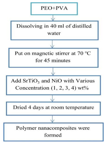
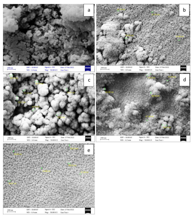
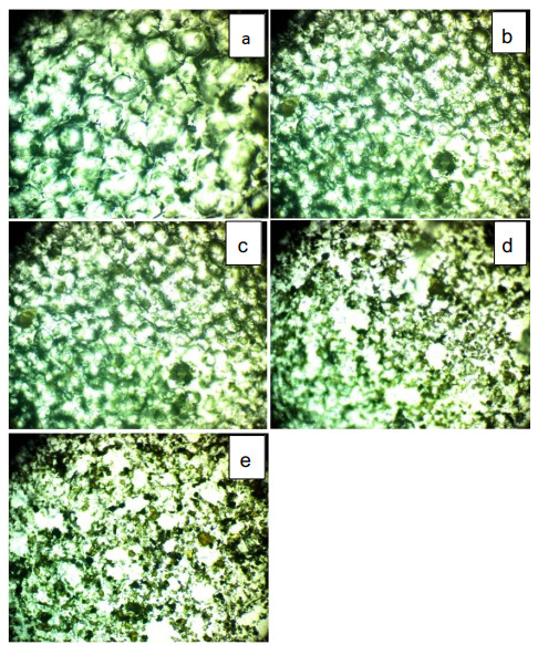
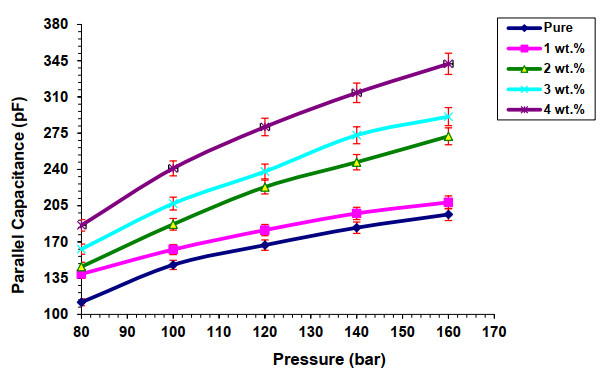
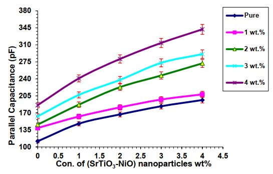
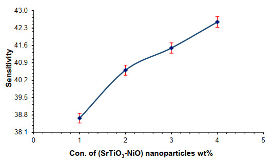
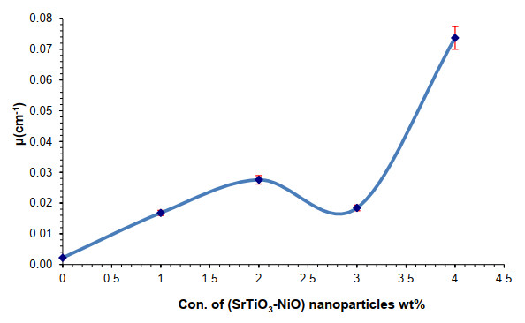
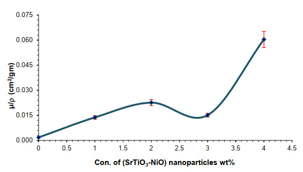
This study looks at the synthesis of innovative PEO/PVA/SrTiO₃/NiO nanocomposites for piezoelectric sensors and gamma shielding applications that are low weight, elastic, affordable and have good gamma ray attenuation coefficients. The impact of SrTiO₃/NiO on the structural characteristics of the PEO/PVA mixture is investigated. The polymer mixture PEO/PVA received additions of SrTiO₃/NiO at concentrations of (0, 1, 2, 3 and 4) weight percent by the casting method. On the top surface of the films PEO/PVA/SrTiO₃/NiO NCs, scanning electron microscopy reveals several randomly distributed aggregates or fragments that are consistent and coherent. An optical microscope image collection reveals that the blend*s additive distribution of NPs was homogenous. Gamma ray shielding application results show that the attenuation coefficient of PVA/PEO/SrTiO₃/NiO NCs is increased by increasing concentration of SrTiO₃/NiO nanoparticles. Radiation protection is another application for it. The pressure sensor application findings of NCs show that, when the applied pressure rises, electrical capacitance (Cp) increase.
- nanocomposites,
- SrTiO₃/CoO NPs,
- piezoelectric sensors,
- gamma ray attenuation
Citation: Shaimaa Mazhar Mahdi, Majeed Ali Habeeb. Low-cost piezoelectric sensors and gamma ray attenuation fabricated from novel polymeric nanocomposites[J]. AIMS Materials Science, 2023, 10(2): 288-300. doi: 10.3934/matersci.2023015

Related Papers:

Abstract

This study looks at the synthesis of innovative PEO/PVA/SrTiO₃/NiO nanocomposites for piezoelectric sensors and gamma shielding applications that are low weight, elastic, affordable and have good gamma ray attenuation coefficients. The impact of SrTiO₃/NiO on the structural characteristics of the PEO/PVA mixture is investigated. The polymer mixture PEO/PVA received additions of SrTiO₃/NiO at concentrations of (0, 1, 2, 3 and 4) weight percent by the casting method. On the top surface of the films PEO/PVA/SrTiO₃/NiO NCs, scanning electron microscopy reveals several randomly distributed aggregates or fragments that are consistent and coherent. An optical microscope image collection reveals that the blend*s additive distribution of NPs was homogenous. Gamma ray shielding application results show that the attenuation coefficient of PVA/PEO/SrTiO₃/NiO NCs is increased by increasing concentration of SrTiO₃/NiO nanoparticles. Radiation protection is another application for it. The pressure sensor application findings of NCs show that, when the applied pressure rises, electrical capacitance (Cp) increase.

References

[1]	Tommasini FJ, Ferreira LdC, Tienne LGP, et al. (2018) Poly(Methyl Methacrylate)-SiC nanocomposites prepared through in situ polymerization. Mat Res 21: e20180086. https://doi.org/10.1590/1980-5373-MR-2018-0086 doi: 10.1590/1980-5373-MR-2018-0086
[2]	Habeeb MA (2011) Effect of rate of deposition on the optical parameters of GaAs films. Eur J Sci Res 57: 478–484.
[3]	Choi B, Park S, Kim S (2015) Preparation of polyethylene oxide composite electrolytes containing imidazoliumcation salt-attached titanium oxides and their conducing behavior. J Ind Eng Chem 31: 352–359. https://doi.org/10.1016/j.jiec.2015.07.009 doi: 10.1016/j.jiec.2015.07.009
[4]	Kumar K, Ravi M, Pavani Y, et al. (2012) Electrical conduction mechanism in NaCl completed PEO/PVP polymer blend electrolytes. J. Non-Cryst Solids 358: 3205–3211. https://doi.org/10.1016/j.jnoncrysol.2012.08.022 doi: 10.1016/j.jnoncrysol.2012.08.022
[5]	Mohammed AH, Habeeb MA (2022) CO₂O₃ nanofiller-based polymer blend nanocomposites for enhanced optical properties for optoelectronics devices and as a model of antibacterial. HIV Nurs 22: 1167–1172. https://doi.org/10.31838/hiv22.02.225 doi: 10.31838/hiv22.02.225
[6]	Habeeb MA (2014) Dielectric and optical properties of (PVAc-PEG-Ber) biocomposites. J Eng Appl Sci 9: 102–108. https://doi.org/10.36478/jeasci.2014.102.108 doi: 10.36478/jeasci.2014.102.108
[7]	Dooley KM, Chen SY, Ross JR (1994) Stable nickel-containing catalysts for the oxidative chupling of methane. J Catal 145: 402–408. https://doi.org/10.1006/jcat.1994.1050 doi: 10.1006/jcat.1994.1050
[8]	Hosseini MA, Malekie S, Kazemi F (2022) Experimental evaluation of gamma radiation shielding characteristics of Polyvinyl Alcohol/Tungsten oxide composite: A comparison study of micro and nano sizes of the fillers. Nucl Instrum Methods Phys Res 1026: 166214. https://doi.org/10.1016/j.nima.2021.166214 doi: 10.1016/j.nima.2021.166214
[9]	Hosseini MA, Zareb H, Malekie S (2023) Raman spectroscopy of electron irradiated Multi-Walled Carbon Nanotube for dosimetry purposes. Radiat Phys Chem 202: 110535. https://doi.org/10.1016/j.radphyschem.2022.110535 doi: 10.1016/j.radphyschem.2022.110535
[10]	Safdari MS, Malekie S, Kashian S, et al. (2022) Introducing a novel beta-ray sensor based on polycarbonate/bismuth oxide nanocomposite. Sci Rep 12: 2496. https://doi.org/10.1038/s41598-022-06544-6 doi: 10.1038/s41598-022-06544-6
[11]	Ebrahimi N, Hosseini MA, Malekie S (2020) Preliminary study of linearity response of γ-irradiated graphene oxide as a novel dosimeter using the Raman spectroscopy. Bull Mater Sci 43: 233. https://doi.org/10.1007/s12034-020-02177-5 doi: 10.1007/s12034-020-02177-5
[12]	Zike ZI, Habeeb MA (2022) Role of BaTiO₃ /TiO₂ nanofillers on the optical characteristics of biopolymer for optics and photonics fields. HIV Nurs 22: 1185–1189. https://doi.org/10.31838/hiv22.02.229 doi: 10.31838/hiv22.02.229
[13]	Shirinov AV, Schomburg WK (2008) Pressure sensor from a PVDF film. Sens Actuators A Phys 142: 48–55. https://doi.org/10.1016/j.sna.2007.04.002 doi: 10.1016/j.sna.2007.04.002
[14]	Janczak D, Słoma M, Wroblewski G, et al. (2014) Screen-printed resistive pressure sensors containing graphene nanoplatelets and carbon nanotubes. Sensors 14: 17304–17312. https://doi.org/10.3390/s140917304 doi: 10.3390/s140917304
[15]	Obaid HN, Habeeb MA, Rashid FL, et al. (2013) Thermal energy storage by nanofluids. J Eng Appl Sci 8: 143–145. https://doi.org/10.36478/jeasci.2013.143.145 doi: 10.36478/jeasci.2013.143.145
[16]	Liao YC, Xu DG, Zhang PC (2018) Preparation and characterization of Bi2O₃/XNBR flexible films for attenuating gamma rays. Nucl Sci Tech 29: 99. https://doi.org/10.1007/s41365-018-0436-7 doi: 10.1007/s41365-018-0436-7
[17]	Habeeb MA, Jaber ZS (2022) Enhancement of structural and optical properties of CMC/PAA blend by addition of zirconium carbide nanoparticles for optics and photonics applications. Eur J Phys 4: 176–182. https://doi.org/10.26565/2312-4334-2022-4-18 doi: 10.26565/2312-4334-2022-4-18
[18]	Jebur QM, Hashim A, Habeeb MA (2020) Fabrication, structural and optical properties for (Polyvinyl alcohol-polyethylene oxide iron oxide) nanocomposites. Egypt J Chem 63: 611–623. https://dx.doi.org/10.21608/ejchem.2019.10197.1669 doi: 10.21608/ejchem.2019.10197.1669
[19]	Erdem M, Baykara O, Dogru M, et al. (2010) A novel shielding material prepared from solid waste containing lead for gamma ray. Radiat Phys Chem 79: 917–922. https://doi.org/10.1016/j.radphyschem.2010.04.009 doi: 10.1016/j.radphyschem.2010.04.009
[20]	Mahdi SM (2022) Evaluation of the influence of SrTiO₃ and CoO nanofillers on the structural and electrical polymer blend characteristics for electronic devices. Dig J Nanomater Biostruct 17: 941–948. https://doi.org/10.15251/DJNB.2022.173.941 doi: 10.15251/DJNB.2022.173.941
[21]	Habeeb MA, Hashim A, Hayder N (2020) Structural and optical properties of novel (PS-Cr₂O₃/ZnCoFe₂O₄) nanocomposites for UV and microwave shielding. Egypt J Chem 63: 697–708. https://dx.doi.org/10.21608/ejchem.2019.12439.1774 doi: 10.21608/ejchem.2019.12439.1774
[22]	Atta ER, Zakaria KM, Madbouly AM (2015) Study on polymer clay layered nanocomposites as shielding materials for ionizing radiation. Int J Recent Sci Res 6: 4263–4269.
[23]	Abbas NK, Habeeb MA, Algidsawi AJK (2015) Preparation of chloro penta amine cobalit(Ⅲ) chloride and study of its influence on the structural and some optical properties of polyvinyl acetate. Int J of Polym Sci 2015: 926789. https://doi.org/10.1155/2015/926789 doi: 10.1155/2015/926789
[24]	Hayder N, Habeeb MA, Hashim A (2020) Structural, optical and dielectric properties of (PS-In₂O₃/ZnCoFe₂O₄) nanocomposites. Egypt J Chem 63: 577–592. https://doi.org/10.21608/ejchem.2019.14646.18874 doi: 10.21608/ejchem.2019.14646.18874
[25]	Mahdi SM, Habeeb MA (2022) Synthesis and augmented optical characteristics of PEO-PVA-SrTiO₃-NiO hybrid nanocomposites for optoelectronics and antibacterial applications. Opt Quantum Electron 54: 854. https://doi.org/10.1007/s11082-022-04267-6 doi: 10.1007/s11082-022-04267-6
[26]	Chandra K, Ipsita C, Debdulal S, et al. (2015) Modified clad optical fibre coated with PVA/TiO₂ nanocomposite for humidity sensing application. Int J Smart Sens Intell Syst 8: 1424–1442. https://doi.org/10.21307/ijssis-2017-813 doi: 10.21307/ijssis-2017-813
[27]	Jebur QM, Hashim A, Habeeb MA (2020) Structural, AC electrical and optical properties of (polyvinyl alcohol-polyethylene oxide-aluminum oxide) nanocomposites for piezoelectric devices. Egypt J Chem 63: 719–734. https://dx.doi.org/10.21608/ejchem.2019.14847.1900 doi: 10.21608/ejchem.2019.14847.1900
[28]	Habeeb MA, Hashim A, Hayder N (2020) Fabrication of (PS-Cr₂O₃/ZnCoFe₂O₄) nanocomposites and studying their dielectric and fluorescence properties for IR sensors. Egypt J Chem 63: 709–717. https://dx.doi.org/10.21608/ejchem.2019.13333 doi: 10.21608/ejchem.2019.13333
[29]	Habeeb MA, Abdul Hamza RS (2018) Novel of (biopolymer blend-MgO) nanocomposites: Fabrication and characterization for humidity sensors. J Bionanosci 12: 328–335. https://doi.org/10.1166/jbns.2018.1535 doi: 10.1166/jbns.2018.1535
[30]	George FF, Leon MC, Ayo A, et al. (2010) Metal oxide semi-conductor gas sensors in environmental monitoring. J Sens 10: 5469–5502. https://doi.org/10.3390/s100605469 doi: 10.3390/s100605469
[31]	Habeeb MA, Kadhim WK (2014) Study the optical properties of (PVA-PVAC-Ti) nanocomposites. J Eng Appl Sci 9: 109–113. https://doi.org/10.36478/jeasci.2014.109.113 doi: 10.36478/jeasci.2014.109.113
[32]	Narsimha P, Shilpa J, Syed K, et al. (2006) Electrical and humidity sensing properties of polyaniline/WO₃ composites. Sens Actuators B Chem 114: 599–603. https://doi.org/10.1016/j.snb.2005.06.057 doi: 10.1016/j.snb.2005.06.057
[33]	Geng WC, Li N, Li XT, et al. (2007) Effect of polymerization time on the humidity sensing properties of polypyrrole. Sens Actuators B Chem 125: 114–119. https://doi.org/10.1016/j.snb.2007.01.041 doi: 10.1016/j.snb.2007.01.041
[34]	Hadi AH, Habeeb MA (2021) Effect of CdS nanoparticles on the optical properties of (PVA-PVP) blends. J Mech Eng Res Developments 44: 265–274. https//jmerd.net/03-2021-265-274
[35]	Roy MK, Mahloniya RG, Bajpai J, et al. (2012) Spectroscopic and morphological evaluation of gamma radiation irradiated polypyrole based nanocomposites. J Adv Mater Lett 3: 426–432. https://doi.org/10.5185/amlett.2012.6373 doi: 10.5185/amlett.2012.6373
[36]	Akkurt I, Akyıldırım H, Mavi B, et al. (2010) Gamma-ray shielding properties of concrete including barite at different energies. Prog Nucl Energy 52: 620–623. https://doi.org/10.1016/j.pnucene.2010.04.006 doi: 10.1016/j.pnucene.2010.04.006
[37]	Habeeb MA, Mahdi WS (2019) Characterization of (CMC-PVP-Fe₂O₃) nanocomposites for gamma shielding application. Int J Emerging Trends Eng Res 7: 247–255. https://doi.org/10.30534/ijeter/2019/06792019 doi: 10.30534/ijeter/2019/06792019
[38]	Habeeb MA, Hamza RSA (2018) Synthesis of (Polymer blend-MgO) nanocomposites and studying electrical properties for piezoelectric application. Indones J Electr Eng Inf 6: 428–435. https://doi.org/10.11591/ijeei.v6i1.511 doi: 10.11591/ijeei.v6i1.511
[39]	Kaur S, Singh KJ (2013) Comparative study of lead borate and lead silicate glass systems doped with aluminum oxide as gamma-ray shielding materials. Int J Innov Technol Explor Eng 25: 172–175.
[40]	Hashim A, Habeeb MA, Jebur QM (2019) Structural, dielectric and optical properties for (Polyvinyl alcohol-polyethylene oxide manganese oxide) nanocomposites. Egypt J Chem 63: 735–749. https://dx.doi.org/10.21608/ejchem.2019.14849.1901 doi: 10.21608/ejchem.2019.14849.1901
[41]	Zhang J, Yu J, Jaroniec M, et al. (2012) Noble metal-free reduced graphene oxide-Zn_xCd_1-xS nanocomposite with enhanced solar photocatalytic H₂-production performance. Nano Lett 12: 4584–4589. https://doi.org/10.1021/nl301831h doi: 10.1021/nl301831h
[42]	Hadi AH, Habeeb MA (2021) The dielectric properties of (PVA-PVP-CdS) nanocomposites for gamma shielding applications. J Phys Conf Ser 1973: 012063. https://doi.org/10.1088/1742-6596/1973/1/012063 doi: 10.1088/1742-6596/1973/1/012063
[43]	Mahdi SM, Habeeb MA (2022) Fabrication and tailored structural and dielectric characteristics of (SrTiO₃/NiO) nanostructure doped (PEO/PVA) polymeric blend for electronics fields. Phys Chem Solid State 23: 785–792. https://doi.org/10.15330/pcss.23.4.785-792 doi: 10.15330/pcss.23.4.785-792
[44]	Mehrara R, Malekie S, Kotahi SMS, et al. (2021) Introducing a novel low energy gamma ray shield utilizing Polycarbonate Bismuth Oxide composite. Sci Rep 11: 10614. https://doi.org/10.1038/s41598-021-89773-5

Reader Comments

Your name:*

Email:*
© 2023 the Author(s), licensee AIMS Press. This is an open access article distributed under the terms of the Creative Commons Attribution License (http://creativecommons.org/licenses/by/4.0)