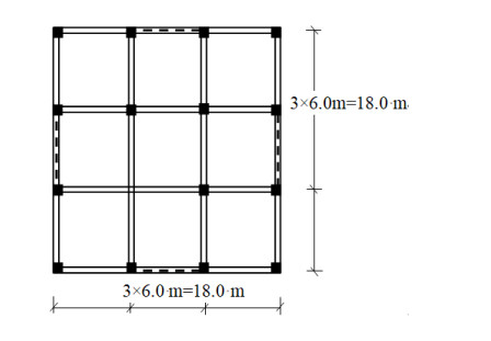
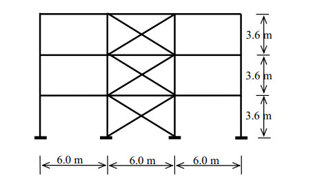
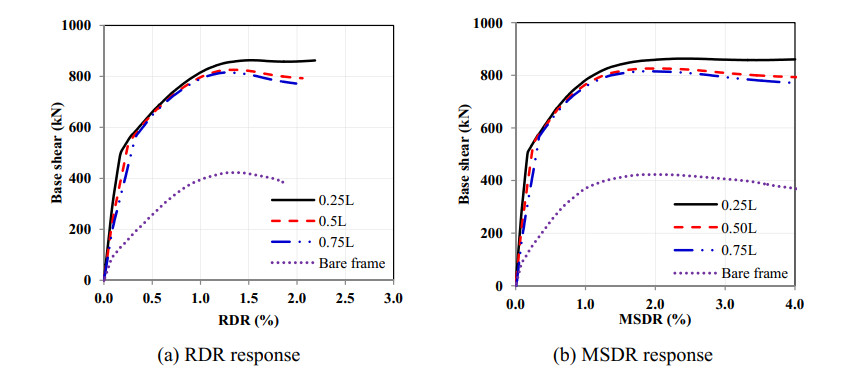
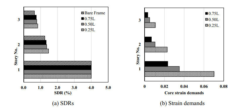
Buckling-restrained braces (BRBs) have proven to be a valuable earthquake resisting system. They demonstrated substantial ability in providing structures with ductility and energy dissipation. However, they are prone to exhibit large residual deformations after earthquake loading because of their low post-yield stiffnesses. In this study, the seismic response of RC frames equipped with BRBs has been investigated. The focus of this research work is on evaluating the effect of the BRB yielding-core length on both the maximum and the residual lateral deformations of the braced RC frames. This is achieved by performing inelastic static pushover and dynamic time-history analyses on three- and nine-story X-braced RC frames having yielding-core length ratios of 25%, 50%, and 75% of the total brace length. The effects of the yielding-core length on both the maximum and the residual lateral deformations of the braced RC frames have been evaluated. Also, the safety of the short-yielding-core BRBs against fracture failures has been checked. An empirical equation has been derived for estimating the critical length of the BRB yielding cores. The results indicated that the high strain hardening capability of reduced length yielding-cores improves the post-yield stiffness and consequently reduces the maximum and residual drifts of the braced RC frames.
Citation: Mohamed Meshaly, Hamdy Abou-Elfath. Seismic response of RC frames equipped with buckling-restrained braces having different yielding lengths[J]. AIMS Materials Science, 2022, 9(3): 359-381. doi: 10.3934/matersci.2022022
Buckling-restrained braces (BRBs) have proven to be a valuable earthquake resisting system. They demonstrated substantial ability in providing structures with ductility and energy dissipation. However, they are prone to exhibit large residual deformations after earthquake loading because of their low post-yield stiffnesses. In this study, the seismic response of RC frames equipped with BRBs has been investigated. The focus of this research work is on evaluating the effect of the BRB yielding-core length on both the maximum and the residual lateral deformations of the braced RC frames. This is achieved by performing inelastic static pushover and dynamic time-history analyses on three- and nine-story X-braced RC frames having yielding-core length ratios of 25%, 50%, and 75% of the total brace length. The effects of the yielding-core length on both the maximum and the residual lateral deformations of the braced RC frames have been evaluated. Also, the safety of the short-yielding-core BRBs against fracture failures has been checked. An empirical equation has been derived for estimating the critical length of the BRB yielding cores. The results indicated that the high strain hardening capability of reduced length yielding-cores improves the post-yield stiffness and consequently reduces the maximum and residual drifts of the braced RC frames.

| [1] | Iwata Y, Sugimoto H, Kuwamura H (2006) Reparability limit of steel buildings based on the actual data of the Hyogoken-Nanbu earthquake, Proceedings of the 38th Joint Panel. Wind and Seismic effects, NIST Special Publication, 1057: 23-32. |
| [2] | McCormick J, Aburano H, Ikenaga M, et al. (2008) Permissible residual deformation levels for building structures considering both safety and human elements, Proceedings of the 14th world conference on earthquake engineering, China: Seismological Press Beijing, 12-17. |
| [3] |
Kasai K, Fu Y, Watanabe A (1998) Passive control systems for seismic damage mitigation. J Struct Eng 124: 501-512. https://doi.org/10.1061/(ASCE)0733-9445(1998)124:5(501) doi: 10.1061/(ASCE)0733-9445(1998)124:5(501)

|
| [4] | Black CJ, Makris N, Aiken ID (2002) Component testing, stability analysis and characterization of buckling-restrained braces. PEER 2002/08, Pacific Earthquake Engineering Research Center, University of California, Berkeley. |
| [5] |
Fahnestock LA, Sause R, Ricles JM, et al. (2003) Ductility demands on buckling restrained braced frames under earthquake loading. Earthq Eng Eng Vib 2: 255-268. https://doi.org/10.1007/s11803-003-0009-5 doi: 10.1007/s11803-003-0009-5
|
| [6] |
Sabelli R, Mahin S, Chang C (2003) Seismic demands on steel braced frame buildings with buckling-restrained braces. Eng Struct 25: 655-666. https://doi.org/10.1016/S0141-0296(02)00175-X doi: 10.1016/S0141-0296(02)00175-X
|
| [7] | Newell J, Uang CM, Benzoni G (2006) Subassemblage testing of core brace buckling restrained braces (G Series). TR-06/01, University of California, San Diego. |
| [8] |
Tremblay R, Bolduc P, Neville R, et al. (2006) Seismic testing and performance of buckling restrained bracing systems. Can J Civil Eng 33: 183-198. https://doi.org/10.1139/l05-103 doi: 10.1139/l05-103
|
| [9] |
Naghavi M, Rahnavard R, Robert J (2019) Numerical evaluation of the hysteretic behavior of concentrically braced frames and buckling restrained brace frame systems. J Build Eng 22: 415-428. https://doi.org/10.1016/j.jobe.2018.12.023 doi: 10.1016/j.jobe.2018.12.023
|
| [10] |
MacRae G, Kimura Y, Roeder C (2004) Effect of column stiffness on braced frame seismic behavior. J Struct Eng 130: 381-391. https://doi.org/10.1061/(ASCE)0733-9445(2004)130:3(381) doi: 10.1061/(ASCE)0733-9445(2004)130:3(381)
|
| [11] |
Zaruma S, Fahnestock LA (2018) Assessment of design parameters influencing seismic collapse performance of buckling restrained braced frames. Soil Dyn Earthq Eng 113: 35-46. https://doi.org/10.1016/j.soildyn.2018.05.021 doi: 10.1016/j.soildyn.2018.05.021
|
| [12] |
Kiggins S, Uang CM (2006) Reducing residual drift of buckling-restrained braced frames as a dual system. Eng Struct 28: 1525-1532. https://doi.org/10.1016/j.engstruct.2005.10.023 doi: 10.1016/j.engstruct.2005.10.023
|
| [13] |
Erochko J, Christopoulos C, Tremblay R, et al. (2011) Residual drift response of SMRFs and BRB Frames in steel buildings designed according to ASCE 7-05. J Struct Eng 137: 589-599. https://doi.org/10.1061/(ASCE)ST.1943-541X.0000296 doi: 10.1061/(ASCE)ST.1943-541X.0000296
|
| [14] |
Ariyaratana CA, Fahnestock LA (2011) Evaluation of buckling-restrained braced frame seismic performance considering reserve strength. Eng Struct 33: 77-89. https://doi.org/10.1016/j.engstruct.2010.09.020 doi: 10.1016/j.engstruct.2010.09.020
|
| [15] |
Hoveidae N, Tremblay R, Rafezy B, et al. (2015) Numerical investigation of seismic behavior of short-core all-steel buckling restrained braces. J Constr Steel Res 114: 89-99. https://doi.org/10.1016/j.jcsr.2015.06.005 doi: 10.1016/j.jcsr.2015.06.005
|
| [16] |
Pandikkadavath M, Sahoo DR (2016) Analytical investigation on cyclic response of buckling-restrained braces with short yielding core segments. Int J Steel Struct 16: 1273-1285. https://doi.org/10.1007/s13296-016-0083-y doi: 10.1007/s13296-016-0083-y
|
| [17] |
Hoveidae N, Radpour S (2021) A novel all-steel buckling restrained brace for seismic drift mitigation of steel frames. B Earthq Eng 19: 1537-1567. https://doi.org/10.1007/s10518-020-01038-0 doi: 10.1007/s10518-020-01038-0
|
| [18] |
Mazzolani F (2008) Innovative metal systems for seismic upgrading of RC structures. J Constr Steel Res 64: 882-895. https://doi.org/10.1016/j.jcsr.2007.12.017 doi: 10.1016/j.jcsr.2007.12.017
|
| [19] | Yooprasertchai E, Warnitchai P (2008) Seismic retrofitting of low-rise nonductile reinforced concrete buildings by buckling-restrained braces, Proceedings of 14th World Conference on Earthquake Engineering, Beijing. |
| [20] | Dinu F, Bordea S, Dubina D (2011) Strengthening of non-seismic reinforced concrete frames of buckling restrained steel braces, Behaviour of Steel Structures in Seismic Areas, 1 Ed., CRC Press. |
| [21] |
Mahrenholtz C, Lin P, Wu A, et al. (2015) Retrofit of reinforced concrete frames with buckling-restrained braces. Earthqu Eng Struct D 44: 59-78. https://doi.org/10.1002/eqe.2458 doi: 10.1002/eqe.2458
|
| [22] |
Abou-Elfath H, Ramadan M, Alkanai FO (2017) Upgrading the seismic capacity of existing RC buildings using buckling restrained braces. Alex Eng J 56: 251-262. https://doi.org/10.1016/j.aej.2016.11.018 doi: 10.1016/j.aej.2016.11.018
|
| [23] |
Ozcelik R, Erdil EE (2019) Pseudodynamic test of a deficient RC frame strengthened with buckling restrained braces. Earthqu Spectra 35: 1163-1187. https://doi.org/10.1193/122317EQS263M doi: 10.1193/122317EQS263M
|
| [24] |
Al-Sadoon ZA, Saatcioglu M, Palermo D (2020) New buckling-restrained brace for seismically deficient reinforced concrete frames. J Struct Eng 146: 04020082. https://doi.org/10.1061/(ASCE)ST.1943-541X.0002439 doi: 10.1061/(ASCE)ST.1943-541X.0002439
|
| [25] |
Sutcu F, Bal A, Fujishita K, et al. (2020) Experimental and analytical studies of sub‑standard RC frames retrofitted with buckling‑restrained braces and steel frames. B Earthq Eng 18: 2389-2410. https://doi.org/10.1007/s10518-020-00785-4 doi: 10.1007/s10518-020-00785-4
|
| [26] |
Castaldo P, Tubaldi E, Selvi F, et al. (2021) Seismic performance of an existing RC structure retrofitted with buckling restrained braces. J Build Eng 33: 101688. https://doi.org/10.1016/j.jobe.2020.101688 doi: 10.1016/j.jobe.2020.101688
|
| [27] |
Xu ZD, Shen YP, Guo YQ (2003) Semi-active control of structures incorporated with magnetorheological dampers using neural networks. Smart Mater Struct 12: 80-87. https://doi.org/10.1088/0964-1726/12/1/309 doi: 10.1088/0964-1726/12/1/309
|
| [28] |
Dai J, Xu ZD, Gai PP, et al. (2021) Optimal design of tuned mass damper inerter with a Maxwell element for mitigating the vortex-induced vibration in bridges. Mech Syst Signal Pr 148: 107180. https://doi.org/10.1016/j.ymssp.2020.107180 doi: 10.1016/j.ymssp.2020.107180
|
| [29] | American Institute of Steel Construction (AISC) (2016) Seismic provisions for structural steel buildings. ANSI/AISC 341-16. |
| [30] | Dehghani M, Tremblay R (2012) Development of standard dynamic loading protocol for buckling-restrained braced frames. International Specialty Conference on Behaviour of Steel Structures in Seismic Area (STESSA 2012), Santiago de Chile |
| [31] | Razavi, SA, Mirghaderi, SR, Seini, A, et al. (2012) Reduced length buckling restrained brace using steel plates as restraining segment, Proceedings of the 15th World Conference on Earthquake Engineering, Lisbon, Portugal. |
| [32] | Nakamura H, Maeda Y, Sasaki T, et al. (2000) Fatigue properties of practical-scale unbonded braces. Nippon Steel Tech Rep 82: 51-57. |
| [33] |
Miner MA (1945) Cumulative damage in fatigue. J Appl Mech 12: 159-164. https://doi.org/10.1115/1.4009458 doi: 10.1115/1.4009458
|
| [34] |
Usami T, Wang C, Funayama J (2011) Low-cycle fatigue tests of a type of buckling restrained braces. Procedia Eng 14: 956-964. https://doi.org/10.1016/j.proeng.2011.07.120 doi: 10.1016/j.proeng.2011.07.120
|
| [35] |
Tabatabaei SAR, Mirghaderi SR, Hosseini A (2014) Experimental and numerical developing of reduced length buckling-restrained braces. Eng Struct 77: 143-160. https://doi.org/10.1016/j.engstruct.2014.07.034 doi: 10.1016/j.engstruct.2014.07.034
|
| [36] |
Pandikkadavath MS, Sahoo DR (2020) Development and subassemblage cyclic testing of hybrid buckling-restrained steel braces. Earthq Eng Eng Vib 19: 967-983. https://doi.org/10.1007/s11803-020-0607-5 doi: 10.1007/s11803-020-0607-5
|
| [37] | Sabelli R (2001) Research on Improving the Design and Analysis of Earthquake-Resistant Steel Braced Frames, California: Earthquake Engineering Research Institute. |
| [38] | SeismoStruct, 2022. A computer program for static and dynamic nonlinear analysis of framed structures. Available from: http://www.seismosoft.com/SeismoStruct. |
| [39] |
Mander JB, Priestley MJN, Park R (1988) Theoretical stress-strain model for confined concrete. J Struct Eng 114: 1804-1826. https://doi.org/10.1061/(ASCE)0733-9445(1988)114:8(1804) doi: 10.1061/(ASCE)0733-9445(1988)114:8(1804)
|
| [40] |
Martinez-Rueda JE, Elnashai AS (1997) Confined concrete model under cyclic load. Mater Struct 30: 139-147. https://doi.org/10.1007/BF02486385 doi: 10.1007/BF02486385
|
| [41] | American Concrete Institute (ACI) Committee 318 (2019) Building code requirements for structural concrete. ACI 318-19. |
| [42] | International code council (2018) 2018 International Building Code. Available from: https://codes.iccsafe.org/content/IBC2018/copyright. |
| [43] | Kiggins K, Uang CM (2006) Reducing residual drift of buckling-restrained braced frames as a dual system. Eng Struct 28: 1525-1532. https://doi.org/10.1016/j.engstruct.2005.10.023 |
| [44] |
Kiggins K and Uang CM (2006) Reducing residual drift of buckling-restrained braced frames as a dual system. Eng Struct 28: 1525-1532. https://doi.org/10.1016/j.engstruct.2005.10.023 doi: 10.1016/j.engstruct.2005.10.023
|
| [45] |
Vamvatsikos D, Cornell CA (2004) Applied incremental dynamic analysis. Earthq Spectra 20: 523-553. https://doi.org/10.1193/1.1737737 doi: 10.1193/1.1737737
|
| [46] |
Kitayama S, Constantinou MC (2018) Collapse performance of seismically isolated buildings designed by the procedures of ASCE/SEI 7. Eng Struct 164: 243-258. https://doi.org/10.1016/j.engstruct.2018.03.008 doi: 10.1016/j.engstruct.2018.03.008
|
| [47] |
Kitayama S, Constantinou MC (2019) Probabilistic seismic performance assessment of seismically isolated buildings designed by the procedures of ASCE/SEI 7 and other enhanced criteria. Eng Struct 179: 566-582. https://doi.org/10.1016/j.engstruct.2018.11.014 doi: 10.1016/j.engstruct.2018.11.014
|
| [48] |
Castaldo P, Amendola G (2021) Optimal DCFP bearing properties and seismic performance assessment in nondimensional form for isolated bridges. Earthq Eng Struct D 50: 2442-2461. https://doi.org/10.1002/eqe.3454 doi: 10.1002/eqe.3454
|
| [49] | Castaldo P, Amendola G (2021) Optimal sliding friction coefficients for isolated viaducts and bridges: A comparison study. Struct Control Hlth e2838. https://doi.org/10.1002/stc.2838 |
| [50] | Applied Technology Council (2009) Quantification of Building Seismic Performance Factors, Washington: Federal Emergency Management Agency. |
| [51] | Federal Emergency Management Agency (2000) Prestandard and Commentary for the Seismic Rehabilitation of Buildings, FEMA 356, Washington, DC, USA. |
Figures(16) / Tables(9)

Mohamed Meshaly, Hamdy Abou-Elfath. Seismic response of RC frames equipped with buckling-restrained braces having different yielding lengths[J]. AIMS Materials Science, 2022, 9(3): 359-381. doi: 10.3934/matersci.2022022


 DownLoad: