Study on the spatial variation of sensitivity of soil nutrient system in Xinjiang, China

Yang Sheng; Dehua Sun; Weizhong Liu; Yang Sheng; Dehua Sun; Weizhong Liu

doi:10.3934/geosci.2023034

AIMS Geosciences

2023, Volume 9, Issue 4: 632-651. doi: 10.3934/geosci.2023034

Previous Article Next Article

Theory article Special Issues

Study on the spatial variation of sensitivity of soil nutrient system in Xinjiang, China

1.
School of Economy and Management, Xinjiang University, Urumchi 830000, China
2.
Arid Region Rural Development Resarch Center, Xinjiang Agricultural University, Urumchi 830052, China

Received: 11 January 2023 Revised: 18 September 2023 Accepted: 25 September 2023 Published: 11 October 2023

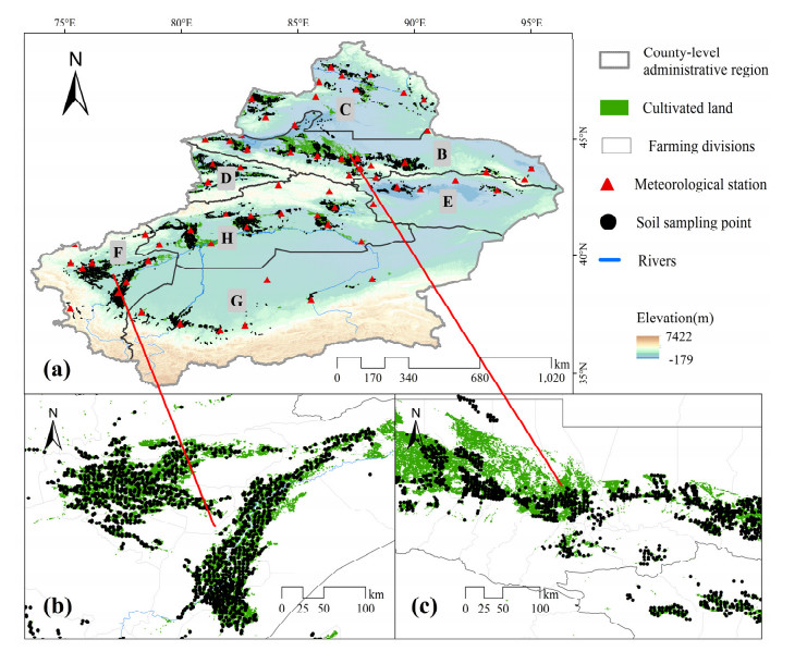
Previous studies have explored the long time series and large-scale cultivated land nutrient sensitivity and its spatial differentiation characteristics in arid zones from human activities in the context of climate change. This study is based on 10-year interval data on soil nutrient content of cultivated land in the oasis in Xinjiang, China, cultivated land use intensity (LUI) and climate data sets. Using sensitivity and GIS analysis methods, this paper studies soil nutrient sensitivities and their spatial distribution patterns in the context of LUI and climate change. The results showed significant response differences and spatial heterogeneity regarding the sensitivity of soil nutrient systems to LUI and climate change. Among them, soil nutrients were the most sensitive to temperature changes, followed by LUI, while precipitation was the weakest. Soil nutrient sensitivity showed a decreasing spatial distribution pattern from the northeast to the southwest. The soil nutrient system had a strong adaptability to LUI and climate change. However, there were differences in different sensitivity states. These results provide scientific guidance for the spatial selection and implementation of soil fertility enhancement and land remediation projects in similar arid areas.
- soil nutrients,
- land-use intensity (LUI),
- climate change,
- sensitivity,
- Xinjiang
Citation: Yang Sheng, Dehua Sun, Weizhong Liu. Study on the spatial variation of sensitivity of soil nutrient system in Xinjiang, China[J]. AIMS Geosciences, 2023, 9(4): 632-651. doi: 10.3934/geosci.2023034

Related Papers:

Abstract

Previous studies have explored the long time series and large-scale cultivated land nutrient sensitivity and its spatial differentiation characteristics in arid zones from human activities in the context of climate change. This study is based on 10-year interval data on soil nutrient content of cultivated land in the oasis in Xinjiang, China, cultivated land use intensity (LUI) and climate data sets. Using sensitivity and GIS analysis methods, this paper studies soil nutrient sensitivities and their spatial distribution patterns in the context of LUI and climate change. The results showed significant response differences and spatial heterogeneity regarding the sensitivity of soil nutrient systems to LUI and climate change. Among them, soil nutrients were the most sensitive to temperature changes, followed by LUI, while precipitation was the weakest. Soil nutrient sensitivity showed a decreasing spatial distribution pattern from the northeast to the southwest. The soil nutrient system had a strong adaptability to LUI and climate change. However, there were differences in different sensitivity states. These results provide scientific guidance for the spatial selection and implementation of soil fertility enhancement and land remediation projects in similar arid areas.

References

[1]	Ajayi AE, Faloye OT, Reinsch T, et al. (2021) Changes in soil structure and pore functions under long term/continuous grassland management. Agric Ecosyst Environ 314: 107407. https://doi.org/10.1016/j.agee.2021.107407 doi: 10.1016/j.agee.2021.107407
[2]	Beillouin D, Cardinael R, Berre D, et al. (2022) A global overview of studies about land management, land-use change, and climate change effects on soil organic carbon. Global Change Biol 28: 1690–1702. https://doi.org/10.1111/gcb.15998 doi: 10.1111/gcb.15998
[3]	Jansson JK, Hofmockel KS (2020) Soil microbiomes and climate change. Nat Rev Microbiol 18: 35–46. https://doi.org/10.1038/s41579-019-0265-7 doi: 10.1038/s41579-019-0265-7
[4]	Zwetsloot MJ, van Leeuwen J, Hemerik L, et al. (2021) Soil multifunctionality: Synergies and trade-offs across European climatic zones and land uses. Eur J Soil Sci 72: 1640–1654. https://doi.org/10.1111/ejss.13051 doi: 10.1111/ejss.13051
[5]	Krah K, Michelson H, Perge E, et al. (2019) Constraints to adopting soil fertility management practices in Malawi: A choice experiment approach. World Development 124: 104651. https://doi.org/10.1016/j.worlddev.2019.104651 doi: 10.1016/j.worlddev.2019.104651
[6]	Techen AK, Helming K (2017) Pressures on soil functions from soil management in Germany. A foresight review. Agron Sustain Dev 37: 64. https://doi.org/10.1007/s13593-017-0473-3 doi: 10.1007/s13593-017-0473-3
[7]	Vanlauwe B, Six J, Sanginga N, et al. (2015) Soil fertility decline at the base of rural poverty in sub-Saharan Africa. Nat Plants 1:15101. https://doi.org/10.1038/nplants.2015.101 doi: 10.1038/nplants.2015.101
[8]	Yanai J, Tanaka S, Nakao A, et al. (2021) Long-term changes in paddy soil fertility in tropical Asia after 50 years of the Green Revolution. Eur J Soil Sci 73: e13193. https://doi.org/10.1111/ejss.13193 doi: 10.1111/ejss.13193
[9]	Lessmann M, Ros GH, Young MD, et al. (2022) Global variation in soil carbon sequestration potential through improved cropland management. Global Change Biol 28: 1162–1177. https://doi.org/10.1111/gcb.15954 doi: 10.1111/gcb.15954
[10]	Siqueira-Neto M, Popin GV, Piccolo MC, et al. (2021) Impacts of land use and cropland management on soil organic matter and greenhouse gas emissions in the Brazilian Cerrado. Eur J Soil Sci 72: 1431–1446. https://doi.org/10.1111/ejss.13059 doi: 10.1111/ejss.13059
[11]	Nandan R, Singh V, Singh SS, et al. (2019) Impact of conservation tillage in rice–based cropping systems on soil aggregation, carbon pools and nutrients. Geoderma 340: 104–114. https://doi.org/10.1016/j.geoderma.2019.01.001 doi: 10.1016/j.geoderma.2019.01.001
[12]	Paramesh V, Singh SK, Mohekar DS, et al. (2022) Impact of sustainable land-use management practices on soil carbon storage and soil quality in Goa State, India. Land Degrad Dev 33: 28–40. https://doi.org/10.1002/ldr.4124 doi: 10.1002/ldr.4124
[13]	Prokop P, Kruczkowska B, Syiemlieh HJ, et al. (2018) Impact of topoFigurey and sedentary swidden cultivation on soils in the hilly uplands of North-East India. Land Degrad Dev 29: 2760–2770. https://doi.org/10.1002/ldr.3018 doi: 10.1002/ldr.3018
[14]	Zhang Y, Tan C, Wang R, et al. (2021) Conservation tillage rotation enhanced soil structure and soil nutrients in long-term dryland agriculture. Eur J Agron 131: 126379. https://doi.org/10.1016/j.eja.2021.126379 doi: 10.1016/j.eja.2021.126379
[15]	Bos JFFP, ten Berge HFM, Verhagen J, et al. (2017) Trade-offs in soil fertility management on arable farms. Agric Syst 157: 292–302. https://doi.org/10.1016/j.agsy.2016.09.013 doi: 10.1016/j.agsy.2016.09.013
[16]	Nikolskii YN, Aidarov IP, Landeros-Sanchez C, et al. (2019) Impact of long-term freshwater irrigation on soil fertility. Irrig Drain 68: 993–1001. https://doi.org/10.1002/ird.2381 doi: 10.1002/ird.2381
[17]	Peigné J, Vian JF, Payet V, et al. (2018) Soil fertility after 10 years of conservation tillage in organic farming. Soil Tillage Res 175:194–204. https://doi.org/10.1016/j.still.2017.09.008 doi: 10.1016/j.still.2017.09.008
[18]	Jing X, Chen X, Fang J, et al. (2020) Soil microbial carbon and nutrient constraints are driven more by climate and soil physicochemical properties than by nutrient addition in forest ecosystems. Soil Biol Biochem 141: 107657. https://doi.org/10.1016/j.soilbio.2019.107657 doi: 10.1016/j.soilbio.2019.107657
[19]	Tamene L, Sileshi GW, Ndengu G, et al. (2019) Soil structural degradation and nutrient limitations across land use categories and climatic zones in Southern Africa. Land Degrad Dev 30: 1288–1299. https://doi.org/10.1002/ldr.3302 doi: 10.1002/ldr.3302
[20]	Guillaume T, Maranguit D, Murtilaksono K, et al. (2016) Sensitivity and resistance of soil fertility indicators to land-use changes: New concept and examples from conversion of Indonesian rainforest to plantations. Ecol Indic 67: 49–57. https://doi.org/10.1016/j.ecolind.2016.02.039 doi: 10.1016/j.ecolind.2016.02.039
[21]	Ichinose Y, Nishigaki T, Kilasara M, et al. (2020) Central roles of livestock and land-use in soil fertility of traditional homegardens on Mount Kilimanjaro. Agroforest Syst 94: 1–14. https://doi.org/10.1007/s10457-019-00357-9 doi: 10.1007/s10457-019-00357-9
[22]	Rolando JL, Dubeux Jr JCB, Ramirez DA, et al. (2018) Land Use Effects on Soil Fertility and Nutrient Cycling in the Peruvian High-Andean Puna Grasslands. Soil Sci Soc Am J 82: 463–474. https://doi.org/10.2136/sssaj2017.09.0309 doi: 10.2136/sssaj2017.09.0309
[23]	Sheng Y, Liu W, Xu H, et al. (2021) The Spatial Distribution Characteristics of the Cultivated Land Quality in the Diluvial Fan Terrain of the Arid Region: A Case Study of Jimsar County, Xinjiang, China. Land 10: 896. https://doi.org/10.3390/land10090896 doi: 10.3390/land10090896
[24]	Zhang C, Liu C, Xu X, et al. (2019) Shukun Energetic, exergetic, economic and environmental (4E) analysis and multi-factor evaluation method of low GWP fluids in trans-critical organic Rankine cycles. Energy 168: 332–345. https://doi.org/10.1016/j.energy.2018.11.104 doi: 10.1016/j.energy.2018.11.104
[25]	Gülü Y (2020) Improved visualization for trend analysis by comparing with classical Mann-Kendall test and ITA. J Hydrol 584: 124674. https://doi.org/10.1016/j.jhydrol.2020.124674 doi: 10.1016/j.jhydrol.2020.124674
[26]	Rasouli K, Pomeroy JW, Whitfield PH (2022) The sensitivity of snow hydrology to changes in air temperature and precipitation in three North American headwater basins. J Hydrol 606: 127460. https://doi.org/10.1016/j.jhydrol.2022.127460 doi: 10.1016/j.jhydrol.2022.127460
[27]	Lenhart T, Eckhardt K, Fohrer HG (2022) Comparison of two different approaches of sensitivity analysis. Phys Chem Earth 27: 645–654. https://doi.org/10.1016/S1474-7065(02)00049-9 doi: 10.1016/S1474-7065(02)00049-9
[28]	Ye S, Song C, Shen S, et al. (2020) Spatial pattern of arable land-use intensity in China. Land Use Policy 99: 104845. https://doi.org/10.1016/j.landusepol.2020.104845 doi: 10.1016/j.landusepol.2020.104845
[29]	Neumann K, Verburg PH, Stehfest E, et al. (2010) The yield gap of global grain production: A spatial analysis. Agric Syst 103: 316–326. https://doi.org/10.1016/j.agsy.2010.02.004 doi: 10.1016/j.agsy.2010.02.004
[30]	Zhang SR, Huang YF, Li BG, et al. (2003) Temporal and spatial variability of soil available phosphorus and potassium in the alluvial region of the Huang_Huai_Hai Plain. Plant Nutr Fert Sci 9: 6.
[31]	Qi Y, Wang Y, Fu BJ, et al. (2008) Spatiotemporal variation in soil quality and its relation to the environmental factors. Prog Phys Geogr 27: 9.
[32]	Liu WJ, Chen SY, Hu FZ, et al. (2012) Distributions pattern of phosphorus, potassium and influencing factors in the up-stream of Shule River Basin. Acta Ecol Sin 32: 9. https://doi.org/10.5846/stxb201111211774 doi: 10.5846/stxb201111211774
[33]	Fayiah M, Dong S, Li Y, et al. (2019) The relationships between plant diversity, plant cover, plant biomass and soil fertility vary with grassland type on Qinghai-Tibetan Plateau. Agric Ecosyst Environ 286: 106659. https://doi.org/10.1016/j.agee.2019.106659 doi: 10.1016/j.agee.2019.106659
[34]	Wang L, Ashraf U, Chang C, et al. (2020) Effects of Silicon and Phosphatic Fertilization on Rice Yield and Soil Fertility. J Soil Sci Plant Nutr 20: 557–565. https://doi.org/10.1007/s42729-019-00145-5 doi: 10.1007/s42729-019-00145-5
[35]	Bednar M, Sarapatka B (2018) Relationships between physical-geoFigureical factors and soil degradation on agricultural land. Environ Res 164: 660–668. https://doi.org/10.1016/j.envres.2018.03.042 doi: 10.1016/j.envres.2018.03.042
[36]	Ferreira CSS, Seifollahi-Aghmiuni S, Destouni G, et al. (2022) Soil degradation in the European Mediterranean region: Processes, status and consequences. Sci Total Environ 805: 150106. https://doi.org/10.1016/j.scitotenv.2021.150106 doi: 10.1016/j.scitotenv.2021.150106
[37]	Zaidel'man FR (2009) Degradation of soils as a result of human-induced transformation of their water regime and soil-protective practice. Eurasian Soil Sci 42: 82–92. https://doi.org/10.1134/S1064229309010116 doi: 10.1134/S1064229309010116
[38]	Dong L, Li J, Zhang Y, et al. (2022) Effects of vegetation restoration types on soil nutrients and soil erodibility regulated by slope positions on the Loess Plateau. J Environ 302: 13985. https://doi.org/10.1016/j.jenvman.2021.113985 doi: 10.1016/j.jenvman.2021.113985
[39]	Li G, Kim S, Han SH, et al. (2018) Precipitation affects soil microbial and extracellular enzymatic responses to warming. Soil Biol Biochem 120: 212–221. https://doi.org/10.1016/j.soilbio.2018.02.014 doi: 10.1016/j.soilbio.2018.02.014
[40]	Liu Y, Zhang H, Xiong M, et al. (2017) Abundance and composition response of wheat field soil bacterial and fungal communities to elevated CO₂ and increased air temperature. Biol Fertil 53: 3–8. https://doi.org/10.1007/s00374-016-1159-8 doi: 10.1007/s00374-016-1159-8
[41]	Yan G, Xing Y, Liu G, et al. (2021) Precipitation pattern regulates soil carbon flux responses to nitrogen addition in a temperate forest. Ecosystems 24: 1608–1623. https://doi.org/10.1007/s10021-021-00606-y doi: 10.1007/s10021-021-00606-y
[42]	Shao Y, Xie Y, Wang C, et al. (2016) Effects of different soil conservation tillage approaches on soil nutrients, water use and wheat-maize yield in rainfed dry-land regions of North China. Eur J Agron 81: 37–45. https://doi.org/10.1016/j.eja.2016.08.014 doi: 10.1016/j.eja.2016.08.014
[43]	Yuan ZY, Jiao F, Shi XR, et al. (2017) Experimental and observational studies find contrasting responses of soil nutrients to climate change. ELife 6: e23255. https://doi.org/10.7554/eLife.23255 doi: 10.7554/eLife.23255
[44]	Tschakert P, Sagoe R, Ofori-Darko G, et al. (2010) Floods in the sahel: an analysis of anomalies, memory, and anticipatory learning. Climatic Change 103: 471–502. https://doi.org/10.1007/s10584-009-9776-y doi: 10.1007/s10584-009-9776-y
[45]	Xue Z, Ullrich P (2021) A retrospective and prospective examination of the 1960s u.s. northeast drought. Earth's Future 9: e2020EF001930. https://doi.org/10.1029/2020EF001930 doi: 10.1029/2020EF001930
[46]	Ding JL; Wang F (2017) Environmental modeling of large-scale soil salinity information in an arid region:A case study of the low and middle altitude alluvial plain north and south of the Tianshan Mountains, Xinjiang. Acta Geogr Sin 72: 64–78.
[47]	Gu ML, Liu HL, Li ZQ, et al. (2014) Impact of biochar application on soil nutrients and microbial diversities in continuous cultivated cotton fields in Xinjiang. China Agri Sci 47: 4128–4138.
[48]	Tang GM, Zhang YS, Xu WL, et al. (2020) Effects of long-term cultivation on contents of organic carbon and total nitrogen in soil particulate fraction in oasis farmland of Xinjiang. China Agri Sci 53: 5039–5050.
[49]	Wang CG, Liu Y, Zhang W (2009) Effects of long-term irrigation with brackish groundwater on soil microbial biomass in cotton field in arid oasis. CSAE 25: 44–48.

geosci-09-04-034-s001.pdf

Reader Comments

Your name:*

Email:*
© 2023 the Author(s), licensee AIMS Press. This is an open access article distributed under the terms of the Creative Commons Attribution License (http://creativecommons.org/licenses/by/4.0)