Calculation and determination of radioactivity in the old district of Najaf by using the track detector CR-39 and geographical information systems (GIS) methods

Adil A Mansoor; Hameed M Abduljabbar; Adil A Mansoor; Hameed M Abduljabbar

doi:10.3934/geosci.2022039

AIMS Geosciences

2022, Volume 8, Issue 4: 709-717. doi: 10.3934/geosci.2022039

Previous Article Next Article

Research article Special Issues

Calculation and determination of radioactivity in the old district of Najaf by using the track detector CR-39 and geographical information systems (GIS) methods

Adil A Mansoor ,
Hameed M Abduljabbar ^,

Department of Physics, College of Education for Pure Science Ibn-Al-Haitham, University of Baghdad, Baghdad, Iraq

Received: 24 July 2022 Revised: 03 October 2022 Accepted: 19 October 2022 Published: 26 October 2022

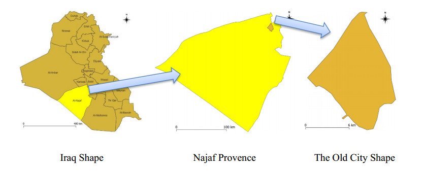
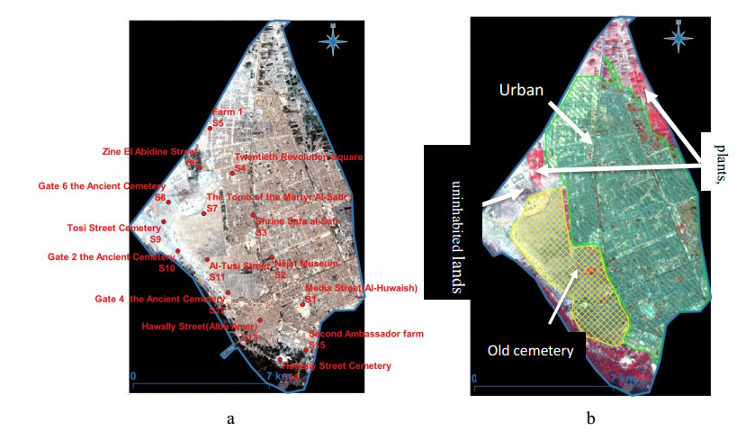
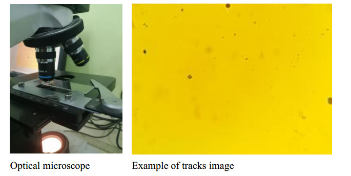
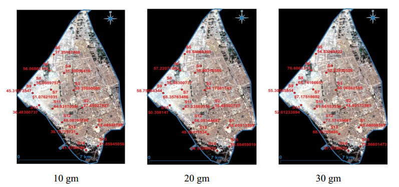
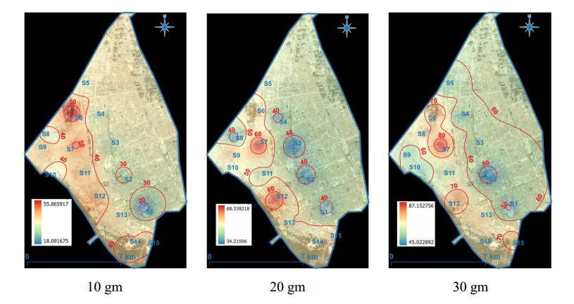
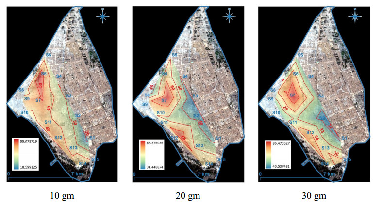
This research aims to study the radiation concentration distribution of the old District of Najaf (Iraq), where 15 samples were taken from featured sites in the District, which represents archaeological, religious, and heritage sites. Track detector CR-39 was used to calculate the concentration of three different soil weights for each sample site after being exposed for a month. Geographical information systems (GIS) were used to distribute the radioactive concentration on the sites of the samples, where two interpolation methods, namely the inverse distance weight method (IDW) and the triangle irregular network method (NIT), to study the distribution of the radioactivity concentration. The study showed that the western part of the district, which includes the old cemetery and the areas adjacent to the Najaf water depression, are characterized by a relatively high amount of radioactivity concentration compared to the eastern part, which represent the residential areas, and for all sample weights.
- radiation,
- radon concentration,
- old district of Najaf,
- CR-39,
- GIS
Citation: Adil A Mansoor, Hameed M Abduljabbar. Calculation and determination of radioactivity in the old district of Najaf by using the track detector CR-39 and geographical information systems (GIS) methods[J]. AIMS Geosciences, 2022, 8(4): 709-717. doi: 10.3934/geosci.2022039

Related Papers:

Abstract

This research aims to study the radiation concentration distribution of the old District of Najaf (Iraq), where 15 samples were taken from featured sites in the District, which represents archaeological, religious, and heritage sites. Track detector CR-39 was used to calculate the concentration of three different soil weights for each sample site after being exposed for a month. Geographical information systems (GIS) were used to distribute the radioactive concentration on the sites of the samples, where two interpolation methods, namely the inverse distance weight method (IDW) and the triangle irregular network method (NIT), to study the distribution of the radioactivity concentration. The study showed that the western part of the district, which includes the old cemetery and the areas adjacent to the Najaf water depression, are characterized by a relatively high amount of radioactivity concentration compared to the eastern part, which represent the residential areas, and for all sample weights.

References

[1]	Hussein DAS, Measurement of Radon Concentrations in College of Education/Ibn Al-Haitham Buildings Using CR-39 Detector and RAD-7 Monitor. Baghdad: College of Education/Ibn Al- Haitham, University of Baghdad, 2018.
[2]	Mahdi KH, Subhi AT, Sharif NR, et al. (2018) Determination of Radon Concentrations in Soil Around Al-Tuwaitha Site Using CR-39 Detector. Eng Technol J 36: 108–112. http://dx.doi.org/10.30684/etj.36.2C.2 doi: 10.30684/etj.36.2C.2
[3]	Saed BM (1998) Determination of radon concentration in buildings by using the nuclear track detector CR-39. College of Education. Ibn Al- Haitham, University of Baghdad.
[4]	Tawfiq NF, Nasir HM, Khalid R (2018) Determination of Radon Concentrations in AL-NAJAF Governorate by Using Nuclear Track Detector CR-39. ANJS 15: 83–87. https://doi.org/10.22401/JNUS.15.1.12 doi: 10.22401/JNUS.15.1.12
[5]	Mohammad GM (1994) Land use mapping of selected areas of county Durham, north-east England, by satellite remote sensing and field survey methods. Durham University.
[6]	Congalton RG, Fenstermaker LK, Ensen JR, et al. (1991) Remote sensing and geographic information system data integration: error sources and Research Issues. Photogramm Eng Remote Sens 57: 677–687.
[7]	Jha MK, Chowdary VM, Peiffer S (2017) Groundwater management and development by integrated remote sensing and geographic information systems: prospects and constraints, CRC Press. Water Resour Manage 21: 427–467. https://doi.org/10.1007/s11269-006-9024-4 doi: 10.1007/s11269-006-9024-4
[8]	Libeesh NK, Naseer KA, Arivazhagan S, et al. (2022) Characterization of Ultramafic–Alkaline–Carbonatite complex for radiation shielding competencies: An experimental and Monte Carlo study with lithological mapping. Ore Geol Rev 142: 104735. https://doi.org/10.1016/j.oregeorev.2022.104735 doi: 10.1016/j.oregeorev.2022.104735
[9]	Alasadi LA, Abojassim AA (2022) Mapping of natural radioactivity in soils of Kufa districts, Iraq using GIS technique. Environ Earth Sci 81: 279. https://doi.org/10.1007/s12665-022-10407-8 doi: 10.1007/s12665-022-10407-8
[10]	Nikezic D, Yu KN (2009) Light scattering from an assembly of tracks in a PADC film. Nucl Instrum Methods Phys Res Sect A 602: 545–551. https://doi.org/10.1016/j.nima.2009.01.204 doi: 10.1016/j.nima.2009.01.204
[11]	Sato F, Kuchimaru T, Kato Y, et al. (2008) Digital image analysis of etch pit formation in CR-39 track detector. Jap J Appl Phys 47: 269–272.
[12]	Mostofizadeh A, Sun X, Kardan MR (2008) Improvement of nuclear track density measurements using image processing techniques. Am J Appl Sci 5: 71–76.
[13]	Tilehnoee Hadad K, Hakimdavoud MR, Hashemi-Tilehnoee M (2011) Indoor radon survey in Shiraz-Iran using developed passive measurement method. Iran J Radiat Res 9: 175–182.
[14]	Yousif SR, Abojassim AA, Hayder A (2019) Mapping of natural radioactivity in soil samples of badra oil field project using GIS program. Nucl Phys Energy 20: 60–69.
[15]	Abduljabbar HM, Abdul IM, Mahdia SH (2018) Measuring surface porosity for zirconium enforced by different additive rates of nanosilica by means of image processing. AIP Conf Proc 1968: 1–8. https://doi.org/10.1063/1.5039231 doi: 10.1063/1.5039231
[16]	Marid HA, Jarallah NT, Abduljabbar HM (2018) Radioactivity effect on the shape ofd even-even nuclei for Uranium and thorium series. Results Phys 11: 406–409. https://doi.org/10.1016/j.rinp.2018.06.024 doi: 10.1016/j.rinp.2018.06.024
[17]	Mahdi KH (2006) Identification and Measurements of Natural and Industrial Radioactive Pollutants in Environment of Baghdad City Using Gamma Spectrometry and Solid State Nuclear Track Detector CR-39. Baghdad: College of Education/Ibn Al- Haitham, Baghdad University.
[18]	Subhi AT (2013) Calculation of the concentrations of depleted uranium in the diyala river sediment samples using the nuclear track detector CR-39. Ibn Al-Haytham J Pure Appl Sci 26: 122–131.
[19]	Mohammed NA, Calculation of the Specific Activity of Radionuclides in Soil and Radon Concentration and its Health Effects in, Baghdad: Collage of Education for Pure Science-Ibn Al Haitham, University of Baghdad, 2020.
[20]	Ishnayyin HG, Find an Empirical Formula for Indoor Radon Measurement Emitting from Building Materials. Baghdad: College of Education/Ibn Al- Haitham, Baghdad University, 2015.

Reader Comments

Your name:*

Email:*
© 2022 the Author(s), licensee AIMS Press. This is an open access article distributed under the terms of the Creative Commons Attribution License (http://creativecommons.org/licenses/by/4.0)