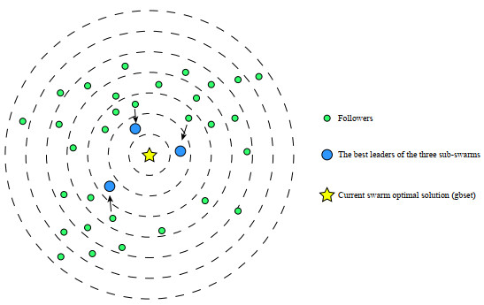
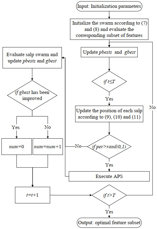
Feature selection (FS) is a promising pre-processing step before performing most data engineering tasks. The goal of it is to select the optimal feature subset with promising quality from the original high-dimension feature space. The Salp Swarm Algorithm (SSA) has been widely used as the optimizer for FS problems. However, with the increase of dimensionality of original feature sets, the FS problems propose significant challenges for SSA. To solve these issues that SSA is easy to fall into local optimum and have poor convergence performance, we propose a multi-swarm SSA (MSSA) to solve the FS problem. In MSSA, the salp swarm was divided into three sub-swarms, the followers updated their positions according to the optimal leader of the corresponding sub-swarm. The design of multi-swarm and multi-exemplar were beneficial to maintain the swarm diversity. Moreover, the updating models of leaders and followers were modified. The salps learn from their personal historical best positions, which significantly improves the exploration ability of the swarm. In addition, an adaptive perturbation strategy (APS) was proposed to improve the exploitation ability of MSSA. When the swarm stagnates, APS will perform the opposition-based learning with the lens imaging principle and the simulated binary crossover strategy to search for promising solutions. We evaluated the performance of MSSA by comparing it with 14 representative swarm intelligence algorithms on 10 well-known UCI datasets. The experimental results showed that the MSSA can obtain higher convergence accuracy with a smaller feature subset.
Citation: Bo Wei, Xiao Jin, Li Deng, Yanrong Huang, Hongrun Wu. Feature selection via a multi-swarm salp swarm algorithm[J]. Electronic Research Archive, 2024, 32(5): 3588-3617. doi: 10.3934/era.2024165
Feature selection (FS) is a promising pre-processing step before performing most data engineering tasks. The goal of it is to select the optimal feature subset with promising quality from the original high-dimension feature space. The Salp Swarm Algorithm (SSA) has been widely used as the optimizer for FS problems. However, with the increase of dimensionality of original feature sets, the FS problems propose significant challenges for SSA. To solve these issues that SSA is easy to fall into local optimum and have poor convergence performance, we propose a multi-swarm SSA (MSSA) to solve the FS problem. In MSSA, the salp swarm was divided into three sub-swarms, the followers updated their positions according to the optimal leader of the corresponding sub-swarm. The design of multi-swarm and multi-exemplar were beneficial to maintain the swarm diversity. Moreover, the updating models of leaders and followers were modified. The salps learn from their personal historical best positions, which significantly improves the exploration ability of the swarm. In addition, an adaptive perturbation strategy (APS) was proposed to improve the exploitation ability of MSSA. When the swarm stagnates, APS will perform the opposition-based learning with the lens imaging principle and the simulated binary crossover strategy to search for promising solutions. We evaluated the performance of MSSA by comparing it with 14 representative swarm intelligence algorithms on 10 well-known UCI datasets. The experimental results showed that the MSSA can obtain higher convergence accuracy with a smaller feature subset.

| [1] |
M. Rostami, K. Berahmand, E. Nasiri, S. Forouzandeh, Review of swarm intelligence-based feature selection methods, Eng. Appl. Artif. Intell., 100 (2021), 104210. https://doi.org/10.1016/j.engappai.2021.104210 doi: 10.1016/j.engappai.2021.104210

|
| [2] |
B. H. Nguyen, B. Xue, M. Zhang, A survey on swarm intelligence approaches to feature selection in data mining, Swarm Evol. Comput., 54 (2020), 100663. https://doi.org/10.1016/j.swevo.2020.100663 doi: 10.1016/j.swevo.2020.100663
|
| [3] |
C. H. Chen, A hybrid intelligent model of analyzing clinical breast cancer data using clustering techniques with feature selection, Appl. Soft Comput., 20 (2014), 4–14. https://doi.org/10.1016/j.asoc.2013.10.024 doi: 10.1016/j.asoc.2013.10.024
|
| [4] |
H. L. Chen, B. Yang, J. Liu, D. Y. Liu, A support vector machine classifier with rough set-based feature selection for breast cancer diagnosis, Expert Syst. Appl., 38 (2011), 9014–9022. https://doi.org/10.1016/j.eswa.2011.01.120 doi: 10.1016/j.eswa.2011.01.120
|
| [5] | S. Tounsi, I. F. Kallel, M. Kallel, Breast cancer diagnosis using feature selection techniques, in 2022 2nd International Conference on Innovative Research in Applied Science, Engineering and Technology (IRASET), IEEE, (2022), 1–5. https://doi.org/110.1109/IRASET52964.2022.9738334 |
| [6] |
B. Sowan, M. Eshtay, K. Dahal, H. Qattous, L. Zhang, Hybrid PSO feature selection-based association classification approach for breast cancer detection, Neural Comput. Appl., 47 (2023), 5291–5317. https://doi.org/10.1007/s00521-022-07950-7 doi: 10.1007/s00521-022-07950-7
|
| [7] |
K. Koras, D. Juraeva, J. Kreis, J. Mazur, E. Staub, E. Szczurek, Feature selection strategies for drug sensitivity prediction, Sci. Rep., 10 (2020), 9377. https://doi.org/10.1038/s41598-020-65927-9 doi: 10.1038/s41598-020-65927-9
|
| [8] |
Z. Zhao, G. Fu, S. Liu, K. M. Elokely, R. J. Doerksen, Y. Chen, et al., Drug activity prediction using multiple-instance learning via joint instance and feature selection, BMC Bioinf., 14 (2013), 1–12. https://doi.org/10.1186/1471-2105-14-S14-S16 doi: 10.1186/1471-2105-14-S14-S16
|
| [9] |
M. Al-Ayyoub, Y. Jararweh, A. Rabab'ah, M. Aldwairi, Feature extraction and selection for Arabic tweets authorship authentication, J. Amb. Intell. Hum. Comput., 8 (2017), 383–393. https://doi.org/10.1007/s12652-017-0452-1 doi: 10.1007/s12652-017-0452-1
|
| [10] |
G. Wang, F. Zhang, Z. Li, Multiview feature selection with information complementarity and consensus for fault diagnosis, IEEE Trans. Syst. Man Cybern.: Syst., 53 (2023), 5058–5070. https://doi.org/110.1109/TSMC.2023.3260100 doi: 10.1109/TSMC.2023.3260100
|
| [11] |
Z. Wang, H. Huang, Y. Wang, Fault diagnosis of planetary gearbox using multi-criteria feature selection and heterogeneous ensemble learning classification, Measurement, 173 (2021), 108654. https://doi.org/10.1016/j.measurement.2020.108654 doi: 10.1016/j.measurement.2020.108654
|
| [12] |
T. Dokeroglu, A. Deniz, H. E. Kiziloz, A comprehensive survey on recent metaheuristics for feature selection, Neurocomputing, 494 (2022), 269–296. https://doi.org/10.1016/j.neucom.2022.04.083 doi: 10.1016/j.neucom.2022.04.083
|
| [13] |
H. Faris, M. M. Mafarja, A. A. Heidari, I. Aljarah, A. Z. Ala'm, S. Mirjalili, et al., An efficient binary Salp Swarm Algorithm with crossover scheme for feature selection problems, Knowl.-Based Syst., 154 (2018), 43–67. https://doi.org/10.1016/j.knosys.2018.05.009 doi: 10.1016/j.knosys.2018.05.009
|
| [14] |
X. Wang, F. Wang, Q. He, Y. Guo, A multi-swarm optimizer with a reinforcement learning mechanism for large-scale optimization, Swarm Evol. Comput., (2024), 101486. https://doi.org/10.1016/j.swevo.2024.101486 doi: 10.1016/j.swevo.2024.101486
|
| [15] |
S. Huang, Z. Wang, Y. Ge, F. Wang, A coevolutionary estimation of distribution algorithm based on dynamic differential grouping for mixed-variable optimization problems, Expert Syst. Appl., 245 (2024), 123122. https://doi.org/10.1016/j.eswa.2023.123122 doi: 10.1016/j.eswa.2023.123122
|
| [16] |
S. Li, F. Wang, Q. He, X. Wang, Deep reinforcement learning for multi-objective combinatorial optimization: A case study on multi-objective traveling salesman problem, Swarm Evol. Comput., 83 (2023), 101398. https://doi.org/10.1016/j.swevo.2023.101398 doi: 10.1016/j.swevo.2023.101398
|
| [17] | R. Eberhart, J. Kennedy, A new optimizer using particle swarm theory, in MHS'95. Proceedings of the Sixth International Symposium on Micro Machine and Human Science, IEEE, (1995), 39–43. https://doi.org/10.1109/MHS.1995.494215 |
| [18] |
B. Wei, X. W. Xia, F. Yu, Y. L. Zhang, X. Xu, Multiple adaptive strategies based particle swarm optimization algorithm, Swarm Evol. Comput., 57 (2020), 100731. https://doi.org/10.1016/j.swevo.2020.100731 doi: 10.1016/j.swevo.2020.100731
|
| [19] |
F. Wang, Q. He, S. Li, Solving combinatorial optimization problems with deep neural network: A survey, Tsinghua Sci. Technol., 29 (2024), 1266–1282. https://doi.org/10.26599/TST.2023.9010076 doi: 10.26599/TST.2023.9010076
|
| [20] | M, Dorigo, C. G. Di, Ant colony optimization: a new meta-heuristic, in IEEE Congress on Evolutionary Computation, IEEE, (1999), 1470–1477. https://doi.org/10.1109/CEC.1999.782657 |
| [21] |
J. Wang, Y. Zhang, M. Hong, H. He, S. Huang, A self-adaptive level-based learning artificial bee colony algorithm for feature selection on high-dimensional classification, Soft Comput., 26 (2022), 9665–9687. https://doi.org/10.1007/s00500-022-06826-1 doi: 10.1007/s00500-022-06826-1
|
| [22] |
S. Mirjalili, A. Lewis, The whale optimization algorithm, Adv. Eng. Software, 95 (2016), 51–67. https://doi.org/10.1016/j.advengsoft.2016.01.008 doi: 10.1016/j.advengsoft.2016.01.008
|
| [23] |
S. Mirjalili, S. M. Mirjalili, A. Lewis, Grey wolf optimizer, Adv. Eng. Software, 69 (2014), 46–61. https://doi.org/10.1016/j.advengsoft.2013.12.007 doi: 10.1016/j.advengsoft.2013.12.007
|
| [24] | X. S. Yang, Firefly algorithms for multimodal optimization, in International Symposium on Stochastic Algorithms, Springer, (2009), 169–178. https://doi.org/10.1007/978-3-642-04944-6_14 |
| [25] | D. Karaboga, An idea based on honey bee swarm for numerical optimization, in Technical Report-tr06, Erciyes University, Engineering Faculty, Computer Engineering Department, (2005), 1–10. |
| [26] |
S. Mirjalili, A. H. Gandomi, S. Z. Mirjalili, S. Saremi, H. Faris, S. M. Mirjalili, Salp Swarm Algorithm: A bio-inspired optimizer for engineering design problems, Adv. Eng. Software, 114 (2017), 163–191. https://doi.org/10.1016/j.advengsoft.2017.07.002 doi: 10.1016/j.advengsoft.2017.07.002
|
| [27] |
E. Rashedi, H. Nezamabadi-Pour, S. Saryazdi, BGSA: binary gravitational search algorithm, Nat. Comput., 9 (2010), 727–745. https://doi.org/10.1007/s11047-009-9175-3 doi: 10.1007/s11047-009-9175-3
|
| [28] |
S. Mirjalili, S. M. Mirjalili, X. S. Yang, Binary bat algorithm, Neural Comput. Appl., 25 (2014), 663–681. https://doi.org/10.1007/s00521-013-1525-5 doi: 10.1007/s00521-013-1525-5
|
| [29] |
M. Abdel-Basset, D. El-Shahat, I. El-henawy, V. H. C. de Albuquerque, S. Mirjalili, A new fusion of grey wolf optimizer algorithm with a two-phase mutation for feature selection, Expert Syst. Appl., 139 (2020), 112824. https://doi.org/10.1016/j.eswa.2019.112824 doi: 10.1016/j.eswa.2019.112824
|
| [30] |
F. Wang, X. Wang, S. Sun, A reinforcement learning level-based particle swarm optimization algorithm for large-scale optimization, Inf. Sci., 602 (2022), 298–312. https://doi.org/10.1016/j.ins.2022.04.053 doi: 10.1016/j.ins.2022.04.053
|
| [31] | K. Chen, B. Xue, M. Zhang, F. Zhou, Correlation-guided updating strategy for feature selection in classification with surrogate-assisted particle swarm optimization, IEEE Trans. Evolut. Comput., (2022), 1015–1029. https://doi.org/10.1109/TEVC.2021.3134804 |
| [32] |
M. Ghosh, R. Guha, R. Sarkar, A. Abraham, A wrapper-filter feature selection technique based on ant colony optimization, Neural Comput. Appl., 32 (2020), 7839–7857. https://doi.org/10.1007/s00521-019-04171-3 doi: 10.1007/s00521-019-04171-3
|
| [33] |
Y. Zhang, S. Cheng, Y. Shi, D. W. Gong, X. Zhao, Cost-sensitive feature selection using two-archive multi-objective artificial bee colony algorithm, Expert Syst. Appl., 137 (2019), 46–58. https://doi.org/10.1016/j.eswa.2019.06.044 doi: 10.1016/j.eswa.2019.06.044
|
| [34] |
R. Salgotra, U. Singh, S. Singh, G. Singh, N. Mittal, Self-adaptive salp swarm algorithm for engineering optimization problems, Appl. Math. Modell., 89 (2021), 188–207. https://doi.org/10.1016/j.apm.2020.08.014 doi: 10.1016/j.apm.2020.08.014
|
| [35] |
I. Aljarah, M. Mafarja, A. A. Heidari, H. Faris, Y. Zhang, S. Mirjalili, Asynchronous accelerating multi-leader salp chains for feature selection, Appl. Soft Comput., 71 (2018), 964–979. https://doi.org/10.1016/j.asoc.2018.07.040 doi: 10.1016/j.asoc.2018.07.040
|
| [36] |
G. I. Sayed, G. Khoriba, M. H. Haggag, A novel chaotic salp swarm algorithm for global optimization and feature selection, Appl. Intell., 48 (2018), 3462–3481. https://doi.org/10.1007/s10489-018-1158-6 doi: 10.1007/s10489-018-1158-6
|
| [37] |
M. A. Tawhid, A. M. Ibrahim, Improved salp swarm algorithm combined with chaos, Math. Comput. Simulat., 202 (2022), 113–148. https://doi.org/10.1016/j.matcom.2022.05.029 doi: 10.1016/j.matcom.2022.05.029
|
| [38] | A. Choura, H. Hellara, M. Baklouti, O. Kanoun, Comparative study of different Salp Swarm Algorithm improvements for feature selection applications, in 2021 International Workshop on Impedance Spectroscopy (IWIS), IEEE, (2021), 146–149. https://doi.org/10.1109/IWIS54661.2021.9711897 |
| [39] |
A. E. Hegazy, M. A. Makhlouf, G. S. El-Tawel, Improved salp swarm algorithm for feature selection, J. King Saud Univ.-Comput. Inf. Sci., 32 (2020), 335–344. https://doi.org/10.1016/j.jksuci.2018.06.003 doi: 10.1016/j.jksuci.2018.06.003
|
| [40] | A. D. Tang, T. Han, D. W. Xu, H. Zhou, L. Xie, An improved salp swarm algorithm using Gaussian distribution estimation strategy, J. Syst. Eng. Electron., 44 (2022), 2229–2240. https://www.sys-ele.com/CN/Y2022/V44/I7/2229 |
| [41] |
J. S. Liu, M. M. Yuan, F. Zuo, Global search-oriented adaptive leader salp swarm algorithm, J. Control. Decis., 36 (2021), 2152–2160. https://doi.org/10.13195/j.kzyjc.2020.0090 doi: 10.13195/j.kzyjc.2020.0090
|
| [42] |
H. Zhang, Z. Cai, X. Ye, M. Wang, F. Kuang, H. Chen, et al., A multi-strategy enhanced salp swarm algorithm for global optimization, Eng. Comput., 38 (2022), 1177–1203. https://doi.org/10.1007/s00366-020-01099-4 doi: 10.1007/s00366-020-01099-4
|
| [43] |
G. Yavuz, Diversified position update equation-based SSA with refreshing-gap strategy for global optimization, J. Comput. Sci., 60 (2022), 101597. https://doi.org/10.1016/j.jocs.2022.101597 doi: 10.1016/j.jocs.2022.101597
|
| [44] |
R. A. Ibrahim, A. A. Ewees, D. Oliva, M. Abd Elaziz, S. Lu, Improved salp swarm algorithm based on particle swarm optimization for feature selection, J. Amb. Intell. Hum. Comput., 10 (2019), 3155–3169. https://doi.org/10.1007/s12652-018-1031-9 doi: 10.1007/s12652-018-1031-9
|
| [45] |
M. Qaraad, S. Amjad, N. K. Hussein, M. A. Elhosseini, Large scale salp-based grey wolf optimization for feature selection and global optimization, Neural Comput. Appl., 34 (2022), 8989–90149. https://doi.org/10.1007/s00521-022-06921-2 doi: 10.1007/s00521-022-06921-2
|
| [46] |
A. H. Gandomi, X. S. Yang, Chaotic bat algorithm, J. Comput. Sci., 5 (2014), 224–232. https://doi.org/10.1016/j.jocs.2013.10.002 doi: 10.1016/j.jocs.2013.10.002
|
| [47] | M. J. Zhang, H. Zhang, X. Chen, J. Yang, A grey wolf optimization algorithm based on Cubic mapping and its application, Comput. Eng. Sci., 43 (2021), 2035–2042. http://manu46.magtech.com.cn/ces/EN/Y2021/V43/I11/2035 |
| [48] |
S. Mahdavi, S. Rahnamayan, K. Deb, Opposition based learning: A literature review, Swarm Evol. Comput., 39 (2018), 1–23. https://doi.org/10.1016/j.swevo.2017.09.010 doi: 10.1016/j.swevo.2017.09.010
|
| [49] | H. R. Tizhoosh, Opposition-based learning: a new scheme for machine intelligence, in International Conference on International Conference on Computational Intelligence for Modelling IEEE, (2005), 695–701. https://doi.org/10.1109/CIMCA.2005.1631345 |
| [50] |
F. Yu, Y. X. Li, B. Wei, X. Xu, Z. Y. Zhao, The application of a novel OBL based on lens imaging principle in PSO, Acta Electron. Sin., 42 (2014), 230–235. https://doi.org/10.3969/j.issn.0372-2112.2014.02.004 doi: 10.3969/j.issn.0372-2112.2014.02.004
|
| [51] | L. Yang, C. Yang, Particle swarm optimization with simulated binary crossover, in 2014 Fifth International Conference on Intelligent Systems Design and Engineering Applications, IEEE, (2014), 710–713. https://doi.org/10.1109/ISDEA.2014.161 |
| [52] |
P. Subbaraj, P. N. Rajnarayanan, Optimal reactive power dispatch using self-adaptive real coded genetic algorithm, Electr. Power Syst. Res., 79 (2009), 374–381. https://doi.org/10.1016/j.epsr.2008.07.008 doi: 10.1016/j.epsr.2008.07.008
|
| [53] | Q. Zhu, Q. Lin, J. Chen, P. Huang, A gene-level hybrid crossover operator for multiobjective evolutionary algorithm, in 2015 Second International Conference on Soft Computing and Machine Intelligence (ISCMI), IEEE, (2015), 20–24. https://doi.org/10.1109/ISCMI.2015.25 |
| [54] |
E. Emary, H. M. Zawbaa, A. E. Hassanien, Binary grey wolf optimization approaches for feature selection, Neurocomputing, 172 (2014), 371–381. https://doi.org/10.1016/j.neucom.2015.06.083 doi: 10.1016/j.neucom.2015.06.083
|
| [55] |
D. E. Goldberg, J. H. Holland, Genetic algorithms and machine learning, Mach. Learn., 3 (1988), 95–99. https://doi.org/10.1023/A:1022602019183 doi: 10.1023/A:1022602019183
|
| [56] |
M. Taradeh, M. Mafarja, A. A. Heidari, H. Faris, I. Aljarah, S. Mirjalili, et al., An evolutionary gravitational search-based feature selection, Inf. Sci., 497 (2019), 219–239. https://doi.org/10.1016/j.ins.2019.05.038 doi: 10.1016/j.ins.2019.05.038
|
| [57] |
S. Arora, P. Anand, Binary butterfly optimization approaches for feature selection, Expert Syst. Appl., 116 (2019), 147–160. https://doi.org/10.1016/j.eswa.2018.08.051 doi: 10.1016/j.eswa.2018.08.051
|
| [58] |
M. M. Mafarja, S. Mirjalili, Hybrid whale optimization algorithm with simulated annealing for feature selection, Neurocomputing, 260 (2017), 302–312. https://doi.org/10.1016/j.neucom.2017.04.053 doi: 10.1016/j.neucom.2017.04.053
|
| [59] |
M. A. Awadallah, A. I. Hammouri, M. A. Al-Betar, M. S. Braik, M. Abd Elaziz, Binary Horse herd optimization algorithm with crossover operators for feature selection, Comput. Biol. Med., 141 (2022), 105152. https://doi.org/10.1016/j.compbiomed.2021.105152 doi: 10.1016/j.compbiomed.2021.105152
|
Figures(6) / Tables(10)
Bo Wei, Xiao Jin, Li Deng, Yanrong Huang, Hongrun Wu. Feature selection via a multi-swarm salp swarm algorithm[J]. Electronic Research Archive, 2024, 32(5): 3588-3617. doi: 10.3934/era.2024165


 DownLoad: