Evaluating the environmental impact on connected vehicles during freeway accidents using VISSIM with probe vehicle data

Hyunju Shin; Jieun Ko; Gunwoo Lee; Cheol Oh; Hyunju Shin; Jieun Ko; Gunwoo Lee; Cheol Oh

doi:10.3934/era.2024135

Electronic Research Archive

2024, Volume 32, Issue 4: 2955-2975. doi: 10.3934/era.2024135

Previous Article Next Article

Research article Special Issues

Evaluating the environmental impact on connected vehicles during freeway accidents using VISSIM with probe vehicle data

1.
Department of Smart City Engineering, Hanyang University ERICA, Ansan 15588, Korea
2.
Department of Transportation and Logistics Engineering, Hanyang University ERICA, Ansan 15588, Korea

Received: 28 November 2023 Revised: 08 April 2024 Accepted: 12 April 2024 Published: 18 April 2024

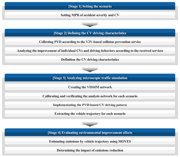
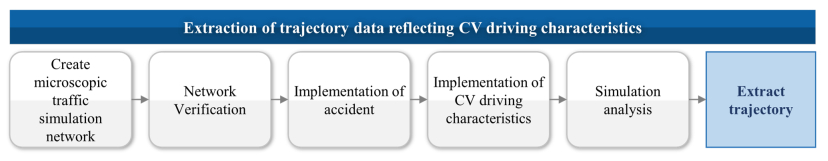
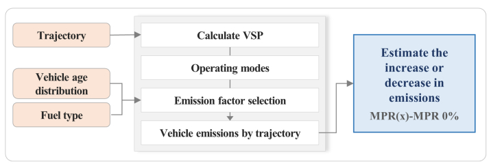
We evaluated emissions as an environmental effect resulting from connected vehicles (CVs) during freeway accidents. The CVs were used to determine the CV driving characteristics, whose values were used to implement the CV driving pattern using a microscopic traffic simulation. The environmental effect of implementation of CV was evaluated using the vehicle trajectory data derived from the simulation results. Implementation of CV effectively minimized the vehicle emissions regardless of the market penetration rate (MPR). In terms of vehicle type, the emissions reduction rate of passenger cars was the highest at a maximum of 33.4%. In the case of pollutants, the reduction rate of CO based on all vehicles was the highest at a maximum of 28.8%. Overall, we found that the implementation of CV positively affected vehicle emissions reductions, and an MPR of 60% could maximize the vehicle emissions reduction effect.
- connected vehicle,
- traffic simulation,
- vehicle emissions,
- traffic accidents,
- probe vehicle data
Citation: Hyunju Shin, Jieun Ko, Gunwoo Lee, Cheol Oh. Evaluating the environmental impact on connected vehicles during freeway accidents using VISSIM with probe vehicle data[J]. Electronic Research Archive, 2024, 32(4): 2955-2975. doi: 10.3934/era.2024135

Related Papers:

Abstract

We evaluated emissions as an environmental effect resulting from connected vehicles (CVs) during freeway accidents. The CVs were used to determine the CV driving characteristics, whose values were used to implement the CV driving pattern using a microscopic traffic simulation. The environmental effect of implementation of CV was evaluated using the vehicle trajectory data derived from the simulation results. Implementation of CV effectively minimized the vehicle emissions regardless of the market penetration rate (MPR). In terms of vehicle type, the emissions reduction rate of passenger cars was the highest at a maximum of 33.4%. In the case of pollutants, the reduction rate of CO based on all vehicles was the highest at a maximum of 28.8%. Overall, we found that the implementation of CV positively affected vehicle emissions reductions, and an MPR of 60% could maximize the vehicle emissions reduction effect.

References

[1]	N. Lu, N. Cheng, N. Zhang, X. Shen, J. W. Mark, Connected vehicles: solutions and challenges, IEEE Internet Things J., 1 (2014), 289–299. http://doi.org/10.1109/JIOT.2014.2327587 doi: 10.1109/JIOT.2014.2327587
[2]	D. Li, F. Zhu, J. Wu, Y. D. Wong, T. Chen, Managing mixed traffic at signalized intersections: An adaptive signal control and CAV coordination system based on deep reinforcement learning, Expert Syst. Appl., 238 (2024), 121959. http://doi.org/10.1016/j.eswa.2023.121959 doi: 10.1016/j.eswa.2023.121959
[3]	C. Chen, J. Wang, Q. Xu, J. Wang, K. Li, Mixed platoon control of automated and human-driven vehicles at a signalized intersection: Dynamical analysis and optimal control, Transp. Res. Part C Emerging Technol. , 127 (2021), 103138. http://doi.org/10.1016/j.trc.2021.103138 doi: 10.1016/j.trc.2021.103138
[4]	C. Ren, L. Wang, C. Yin, Z. Wang, X. Chen, J. Li, Research on the platoon speed guidance strategy at signalized intersections in the connected vehicle environment, J. Adv. Transp., 2023 (2023), 1–25. http://doi.org/10.1155/2023/9984537 doi: 10.1155/2023/9984537
[5]	D. Li, F. Zhu, T. Chen, Y. D. Wong, C. Zhu, J. Wu, COOR-PLT: A hierarchical control model for coordinating adaptive platoons of connected and autonomous vehicles at signal-free intersections based on deep reinforcement learning, Transp. Res. Part C Emerging Technol., 146 (2023), 103933. http://doi.org/10.1016/j.trc.2022.103933 doi: 10.1016/j.trc.2022.103933
[6]	T. Apostolakis, M. A. Makridis, A. Kouvelas, K. Ampountolas, Energy-based assessment and driving behavior of ACC systems and humans inside platoons, IEEE Trans. Intell. Transp. Syst., 24 (2023), 12726–12735. http://doi.org/10.1109/TITS.2023.3285296 doi: 10.1109/TITS.2023.3285296
[7]	J. Lee, B. Park, Development and evaluation of a cooperative vehicle intersection control algorithm under the connected vehicles environment, IEEE Trans. Intell. Transport. Syst., 13 (2012), 81–90. http://doi.org/10.1109/TITS.2011.2178836 doi: 10.1109/TITS.2011.2178836
[8]	Q. Jin, G. Wu, K. Boriboonsomsin, M. Barth, Platoon-based multi-agent intersection management for connected vehicle, in 16th International IEEE Conference on Intelligent Transportation Systems (ITSC 2013), (2013), 1462–1467. http://doi.org/10.1109/ITSC.2013.6728436
[9]	A. Validi, C. Olaverri-Monreal, Simulation-based impact of connected vehicles in platooning mode on travel time, emissions and fuel consumption, in 2021 IEEE Intelligent Vehicles Symposium (Ⅳ), (2021), 1150–1155. http://doi.org/10.1109/IV48863.2021.9575899
[10]	S. Huang, A. W. Sadek, Y. Zhao, Assessing the mobility and environmental benefits of reservation-based intelligent intersections using an integrated simulator, IEEE Trans. Intell. Transport. Syst., 13 (2012), 1201–1214. http://doi.org/10.1109/TITS.2012.2186442 doi: 10.1109/TITS.2012.2186442
[11]	Y. Zhao, A. Wagh, Y. Hou, K. Hulme, C. Qiao, A. W. Sadek, Integrated traffic-driving-networking simulator for the design of connected vehicle applications: eco-signal case study, J. Intell. Transp. Syst., 20 (2016), 75–87. http://doi.org/10.1080/15472450.2014.889920 doi: 10.1080/15472450.2014.889920
[12]	V. Astarita, V. P. Giofré, D. C. Festa, G. Guido, A. Vitale, Floating car data adaptive traffic signals: A description of the first real-time experiment with 'connected' vehicles, Electronics, 9 (2020), 114. http://doi.org/10.3390/electronics9010114 doi: 10.3390/electronics9010114
[13]	X. J. Liang, S. I. Guler, V. V. Gayah, An equitable traffic signal control scheme at isolated signalized intersections using connected vehicle technology, Transp. Res. Part C Emerging Technol., 110 (2020), 81–97. http://doi.org/10.1016/j.trc.2019.11.005 doi: 10.1016/j.trc.2019.11.005
[14]	S. Mamarikas, Evaluation of the effect of 'Energy Efficient Intersection' system on CO₂ emissions of road transport, M.S. thesis, International Hellenic University, 2015.
[15]	E. Mintsis, E. I. Vlahogianni, E. Mitsakis, S. Ozkul, Evaluation of a cooperative speed advice service implemented along an urban arterial corridor, in 2017 5th IEEE International Conference on Models and Technologies for Intelligent Transportation Systems (MT-ITS), (2017), 232–237. http://doi.org/10.1109/MTITS.2017.8005672
[16]	L. Pariota, L. D. Costanzo, A. Coppola, C. D'Aniello, G. N. Bifulco, Green light optimal speed advisory: a C-ITS to improve mobility and pollution, in 2019 IEEE International Conference on Environment and Electrical Engineering and 2019 IEEE Industrial and Commercial Power Systems Europe (EEEIC /I & CPS Europe), (2019), 1–6. http://doi.org/10.1109/EEEIC.2019.8783573
[17]	E. Mintsis, E. I. Vlahogianni, E. Mitsakis, S. Ozkul, Enhanced speed advice for connected vehicles in the proximity of signalized intersections, Eur. Transport Res. Rev., 13 (2021), 2. http://doi.org/10.1186/s12544-020-00458-y doi: 10.1186/s12544-020-00458-y
[18]	A. Olia, H. Abdelgawad, B. Abdulhai, S. N. Razavi, Assessing the potential impacts of connected vehicles: mobility, environmental, and safety perspectives, J. Intell. Transp. Syst., 20 (2016), 229–243. http://doi.org/10.1080/15472450.2015.1062728 doi: 10.1080/15472450.2015.1062728
[19]	G. A. Ubiergo, W. L. Jin, Mobility and environment improvement of signalized networks through Vehicle-to-Infrastructure (V2I) communications, Transp. Res. Part C Emerging Technol., 68 (2016), 70–82. http://doi.org/10.1016/j.trc.2016.03.010 doi: 10.1016/j.trc.2016.03.010
[20]	Q. Jin, G. Wu, K. Boriboonsomsin, M. Barth, Improving traffic operations using real-time optimal lane selection with connected vehicle technology, in 2014 IEEE Intelligent Vehicles Symposium Proceedings, (2014), 70–75. http://doi.org/10.1109/IVS.2014.6856515
[21]	T. H. Nguyen, J. J. Jung, Swarm intelligence-based green optimization framework for sustainable transportation, Sustainable Cities Soc., 71 (2021), 102947. http://doi.org/10.1016/j.scs.2021.102947 doi: 10.1016/j.scs.2021.102947
[22]	B. Khondaker, L. Kattan, Variable speed limit: A microscopic analysis in a connected vehicle environment, Transp. Res. Part C Emerging Technol., 58 (2015), 146–159. http://doi.org/10.1016/j.trc.2015.07.014 doi: 10.1016/j.trc.2015.07.014
[23]	F. Outay, F. Kamoun, F. Kaisser, D. Alterri, A. Yasar, V2V and V2I communications for traffic safety and CO₂ emission reduction: A performance evaluation, Procedia Comput. Sci., 151 (2019), 353–360. http://doi.org/10.1016/j.procs.2019.04.049 doi: 10.1016/j.procs.2019.04.049
[24]	S. Chandra, F. Camal, A simulation-based evaluation of connected vehicle technology for emissions and fuel consumption, Procedia Eng., 145 (2016), 296–303. http://doi.org/10.1016/j.proeng.2016.04.077 doi: 10.1016/j.proeng.2016.04.077
[25]	S. Chandra, A. Nguyen, Freight truck emissions reductions with connected vehicle technology: A case study with I-710 in California, Case Stud. Transp. Policy, 8 (2020), 920–927. http://doi.org/10.1016/j.cstp.2020.05.010 doi: 10.1016/j.cstp.2020.05.010
[26]	T. Degrande, F. Vannieuwenborg, D. Colle, S. Verbrugge, From ITS to C-ITS highway roadside infrastructure: the handicap of a headstart?, in ITS Biennial Conference 2021, 2021.
[27]	J. M. Bandeira, E. Macedo, P. Fernandes, M. Rodrigues, M. Andrade, M. C. Coelho, Potential pollutant emission effects of connected and automated vehicles in a mixed traffic flow context for different road types, IEEE Open J. Intell. Transp. Syst., 2 (2021), 364–383. http://doi.org/10.1109/OJITS.2021.3112904 doi: 10.1109/OJITS.2021.3112904
[28]	A. Mohammadnazar, R. Arvin, A. J. Khattak, Classifying travelers' driving style using basic safety messages generated by connected vehicles: Application of unsupervised machine learning, Transp. Res. Part C Emerging Technol., 122 (2021), 102917. http://doi.org/10.1016/j.trc.2020.102917 doi: 10.1016/j.trc.2020.102917
[29]	S. Thomas, R. B. Jacko, Stochastic model for estimating impact of highway incidents on air pollution and traffic delay, Transp. Res. Rec., 2011 (2007), 107–115. http://doi.org/10.3141/2011-12 doi: 10.3141/2011-12
[30]	K. Ahn, Microscopic Fuel Consumption and Emission Modeling, Virginia Polytechnic Institute, 1998.
[31]	PTV AG, Ptv Vissim 7 User Manual, 2014. Available from: http://toaz.info/doc-view-3.
[32]	U. S. EPA, MOVES and Mobile Source Emissions Research. Available from: https://www.epa.gov/moves.
[33]	S. Jo, Evolution and considerations of transport services by probe vehicle data collection, Transp. Technol. Policy, 13 (2016), 21–29.
[34]	Korea Expressway Corporation, C-ITS Implementation Project, 2018. Available from: http://www.ex.co.kr.
[35]	Korea Expressway Corporation, Expressway C-ITS Service Implementation Plan, 2019. Available from: http://www.ex.co.kr.
[36]	J. Jang, J. Ko, J. Park, C. Oh, S. Kim, Identification of safety benefits by inter-vehicle crash risk analysis using connected vehicle systems data on Korean freeways, Accid. Anal. Prev., 144 (2020), 105675. http://doi.org/10.1016/j.aap.2020.105675 doi: 10.1016/j.aap.2020.105675
[37]	J. Ko, H. Kim, C. Oh, S. Kim, Impact of V2V warning information on traffic stream performance using microscopic simulation based on real-world connected vehicle driving behavior, IEEE Trans. Intell. Transp. Syst., (2023), 1–14. http://doi.org/10.1109/TITS.2023.3287308 doi: 10.1109/TITS.2023.3287308
[38]	V. E. Balas, M. M. Balas, Driver assisting by inverse time to collision, in 2006 World Automation Congress, (2006), 1–6. http://doi.org/10.1109/WAC.2006.376059
[39]	J. Ko, Development of Design and Evaluation Techniques for In-vehicle Warning Information Systems towards Autonomous Cooperative Driving, Ph.D thesis, Hanyang University, 2024.
[40]	G. Lee, S. I. You, S. G. Ritchie, J. D. Saphores, M. Sangkapichai, R. Jayakrishnan, Environmental impacts of a major freight corridor: A study of I-710 in California, Transp. Res. Rec., 2123 (2009), 119–128. http://doi.org/10.3141/2123-13 doi: 10.3141/2123-13
[41]	J. Koupal, L. Landman, E. Nam, J. Warila, C. Scarbro, E. Glover, et al., MOVES2004 Energy and Emission Inputs Reports, United States Environmental Protection Agency, 2005. Available from: https://nepis.epa.gov/Exe/ZyPURL.cgi?Dockey = P1001DAQ.TXT.
[42]	Ministry of Land, Infrastructure and Transport, Total Registered Motor Vehicles, 2017. Available from: https://stat.molit.go.kr/portal/cate/statView.do?hRsId=58&hFormId=1244&hSelectId=1244&hPoint=00&hAppr=1&hDivEng=&oFileName=&rFileName=&midpath=&sFormId=1244&sStart=2017&sEnd=2017&sStyleNum=562&settingRadio=xlsx.
[43]	S. M. P. Siddharth, G. Ramadurai, Calibration of VISSIM for Indian heterogeneous traffic conditions, Procedia-Social Behav. Sci., 104 (2013), 380–389. http://doi.org/10.1016/j.sbspro.2013.11.13 doi: 10.1016/j.sbspro.2013.11.13
[44]	S. M. Hafram, S. Valery, A. H. Hasim, Calibrating and validation microscopic traffic simulation models VISSIM for enhanced highway capacity planning, Int. J. Eng., 36 (2023), 1509–1519. http://doi.org/10.5829/ije.2023.36.08b.11 doi: 10.5829/ije.2023.36.08b.11
[45]	G. Gomes, A. May, R. Horowitz, Congested freeway microsimulation model using VISSIM, Transp. Res. Rec., 1876 (2004), 71–81. http://doi.org/10.3141/1876-08 doi: 10.3141/1876-08
[46]	N. E. Lownes, R. B. Machemehl, Sensitivity of simulated capacity to modification of VISSIM driver behavior parameters, Transp. Res. Rec., 1988 (2006), 102–110. http://doi.org/10.1177/0361198106198800113 doi: 10.1177/0361198106198800113
[47]	A. Mehar, S. Chandra, S. Velmurugan, Highway capacity through vissim calibrated for mixed traffic conditions, KSCE J. Civ. Eng., 18 (2014), 639–645. http://doi.org/10.1007/s12205-014-0440-3 doi: 10.1007/s12205-014-0440-3
[48]	U. Leyn, P. Vortisch, Calibrating VISSIM for the German highway capacity manual, Transp. Res. Rec., 2483 (2015), 74–79. http://doi.org/10.3141/2483-09 doi: 10.3141/2483-09
[49]	E. Brockfeld, R. D. Kühne, P. Wagner, Calibration and validation of microscopic traffic flow models, Transp. Res. Rec., 1876 (2004), 62–70. http://doi.org/10.3141/1876-07 doi: 10.3141/1876-07
[50]	I. El-Shawarby, K. Ahn, H. Rakha, Comparative field evaluation of vehicle cruise speed and acceleration level impacts on hot stabilized emissions, Transp. Res. Part D Transp. Environ., 10 (2005), 13–30. http://doi.org/10.1016/j.trd.2004.09.002 doi: 10.1016/j.trd.2004.09.002
[51]	K. Lee, Charcteristics for auto driving pattern and exhaust emissions by navigation data, in The 85th Conference of Korean Society of Transportation, Korean Society of Transportation, 2021.
[52]	D. Han, Y. Lee, H. Jang, A study of calculation methodology of vehicle emissions based on driver speed and acceleration behavior, J. Korean Soc. Transp., 29 (2011), 107–120.
[53]	Z. Wadud, D. MacKenzie, P. Leiby, Help or hindrance? The travel, energy and carbon impacts of highly automated vehicles, Transp. Res. Part A Policy Pract., 86 (2016), 1–18. http://doi.org/10.1016/j.tra.2015.12.001 doi: 10.1016/j.tra.2015.12.001
[54]	C. Fiori, V. Arcidiacono, G. Fontaras, M. Makridis, K. Mattas, V. Marzano, et al., The effect of electrified mobility on the relationship between traffic conditions and energy consumption, Transp. Res. Part D Transp. Environ., 67 (2019), 275–290. http://doi.org/10.1016/j.trd.2018.11.018 doi: 10.1016/j.trd.2018.11.018

Reader Comments

Your name:*

Email:*
© 2024 the Author(s), licensee AIMS Press. This is an open access article distributed under the terms of the Creative Commons Attribution License (http://creativecommons.org/licenses/by/4.0)