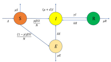
A stochastic continuous-time Markov chain tuberculosis model with fast-slow progression and relapse is established to explore the impact of the demographic variation on TB transmission. At first, the extinction threshold and probability of the disease extinction and outbreak are obtained by applying the multitype Galton-Waston branching process for the stochastic model. In numerical simulations, the probability of the disease extinction and outbreak and expected epidemic duration of the disease are estimated. To see how demographic stochasticity affects TB dynamics, we compare dynamical behaviors of both stochastic and deterministic models, and these results show that the disease extinction in stochastic model would occur while the disease is persistent for the deterministic model. Our results suggest that minimizing the contact between the infectious and the susceptible, and detecting the latently infected as early as possible, etc., could effectively prevent the spread of tuberculosis.
Citation: Tao Zhang, Mengjuan Wu, Chunjie Gao, Yingdan Wang, Lei Wang. Probability of disease extinction and outbreak in a stochastic tuberculosis model with fast-slow progression and relapse[J]. Electronic Research Archive, 2023, 31(11): 7104-7124. doi: 10.3934/era.2023360
A stochastic continuous-time Markov chain tuberculosis model with fast-slow progression and relapse is established to explore the impact of the demographic variation on TB transmission. At first, the extinction threshold and probability of the disease extinction and outbreak are obtained by applying the multitype Galton-Waston branching process for the stochastic model. In numerical simulations, the probability of the disease extinction and outbreak and expected epidemic duration of the disease are estimated. To see how demographic stochasticity affects TB dynamics, we compare dynamical behaviors of both stochastic and deterministic models, and these results show that the disease extinction in stochastic model would occur while the disease is persistent for the deterministic model. Our results suggest that minimizing the contact between the infectious and the susceptible, and detecting the latently infected as early as possible, etc., could effectively prevent the spread of tuberculosis.

| [1] | Overview of Tuberculosis, World Health Organization, 2022. Available from: https://www.who.int/news-room/fact-sheets/detail/tuberculosis. |
| [2] | Global Tuberculosis Report 2022, World Health Organization, 2022. Available from: https://www.who.int/teams/global-tuberculosis-programme/tb-reports/global-tuberculosis-report-2022. |
| [3] |
Z. Feng, C. C. Chavez, A. F. Capurro, A model for tuberculosis with exogenous reinfection, Theor. Popul. Biol., 57 (2000), 235–247. https://doi.org/10.1006/tpbi.2000.1451 doi: 10.1006/tpbi.2000.1451

|
| [4] |
K. D. Dale, M. Karmakar, K. J. Snow, D. Menzies, J. M. Trauer, J. T. Denholm, Quantifying the rates of late reactivation tuberculosis: a systematic review, Lancet Infect. Dis., 21 (2021), 303–317. https://doi.org/10.1016/S1473-3099(20)30728-3 doi: 10.1016/S1473-3099(20)30728-3
|
| [5] |
S. M. Blower, A. R. Mclean, T. C. Porco, P. M. Small, P. C. Hopewell, M. A. Sanchez, et al., The intrinsic transmission dynamics of tuberculosis epidemics, Nat. Med., 1 (1995), 815–821. https://doi.org/10.1038/nm0895-815 doi: 10.1038/nm0895-815
|
| [6] |
E. Ziv, C. L. Daley, S. M. Blower, Early therapy for latent tuberculosis infection, Am. J. Epidemiol., 153 (2002), 381–385. https://doi.org/10.1093/aje/153.4.381 doi: 10.1093/aje/153.4.381
|
| [7] |
M. L. Lambert, E. Hasker, A. V. Deun, D. Roberfroid, M. Boelaert, P. V. D. Stuyft, Recurrence in tuberculosis: relapse or reinfection?, Lancet Infect. Dis., 3 (2003), 281–287. https://doi.org/10.1016/S1473-3099(03)00607-8 doi: 10.1016/S1473-3099(03)00607-8
|
| [8] |
W. S. Avusuglo, R. Mosleh, T. Ramaj, A. Li, S. S. Sharbayta, A. A. Fall, et al., Workplace absenteeism due to COVID-19 and influenza across Canada: A mathematical model, J. Theor. Biol., 572 (2023), 111559. https://doi.org/10.1016/j.jtbi.2023.111559 doi: 10.1016/j.jtbi.2023.111559
|
| [9] |
G. Sun, X. Ma, Z. Zhang, Q. Liu, B. Li, What is the role of aerosol transmission in SARS-Cov-2 Omicron spread in Shanghai?, BMC Infect. Dis., 22 (2022). https://doi.org/10.1186/s12879-022-07876-4 doi: 10.1186/s12879-022-07876-4
|
| [10] |
Y. Tatsukawa, M. R. Arefin, S. Utsumi, K. Kuga, J. Tanimoto, Stochasticity of disease spreading derived from the microscopic simulation approach for various physical contact networks, Appl. Math. Comput., 431 (2022), 127328. https://doi.org/10.1016/j.amc.2022.127328 doi: 10.1016/j.amc.2022.127328
|
| [11] |
X. Ma, G. Sun, Z. Wang, Y. Chu, Z. Jin, B. Li, Transmission dynamics of brucellosis in Jilin province, China: Effects of different control measures, Commun. Nonlinear Sci. Numer. Simul., 114 (2022), 106702. https://doi.org/10.1016/j.cnsns.2022.106702 doi: 10.1016/j.cnsns.2022.106702
|
| [12] |
I. M. Bulai, F. Montefusco, M. G. Pedersen, Stability analysis of a model of epidemic dynamics with nonlinear feedback producing recurrent infection waves, Appl. Math. Lett., 136 (2022), 108455. https://doi.org/10.1016/j.aml.2022.108455 doi: 10.1016/j.aml.2022.108455
|
| [13] |
L. Chang, W. Gong, Z. Jin, G. Sun, Sparse optimal control of pattern formations for an SIR reaction-diffusion epidemic model, SIAM J. Appl. Math., 82 (2022). https://doi.org/10.1137/22M1472127 doi: 10.1137/22M1472127
|
| [14] |
J. Dordevic, B. Jovanovic, Dynamical analysis of a stochastic delayed epidemic model with levy jumps and regime switching, J. Franklin Inst., 36 (2023), 1252–1283. https://doi.org/10.1016/j.jfranklin.2022.12.009 doi: 10.1016/j.jfranklin.2022.12.009
|
| [15] |
G. Sun, H. Zhang, L. Chang, Z. Jin, H. Wang, S. Ruan, On the dynamics of a diffusive Foot-and-Mouth disease model with nonlocal infections, SIAM J. Appl. Math., 82 (2022), 1587–1610. https://doi.org/10.1137/21M1412992 doi: 10.1137/21M1412992
|
| [16] |
S. Y. Tchoumi, M. L. Diagne, H. Rwezaura, J. M. Tchuenche, Malaria and COVID-19 co-dynamics: A mathematical model and optimal control, Appl. Math. Model., 99 (2021), 294–327. https://doi.org/10.1016/j.apm.2021.06.016 doi: 10.1016/j.apm.2021.06.016
|
| [17] |
H. Waaler, A. Geser, S. Andersen, The use of mathematical models in the study of the epidemiology of tuberculosis, Am. J. Public Health, 52 (1962), 1002–1013. https://doi.org/10.2105/AJPH.52.6.1002 doi: 10.2105/AJPH.52.6.1002
|
| [18] |
R. Xu, J. Yang, X. Tian, J. Lin, Global dynamics of a tuberculosis model with fast and slow progression and age-dependent latency and infection, J. Biol. Dyn., 13 (2019), 675–705. https://doi.org/10.1080/17513758.2019.1683628 doi: 10.1080/17513758.2019.1683628
|
| [19] |
C. Liao, Y. Cheng, Y. Lin, H. Hsieh, T. Huang, C. Chio, et al., A probabilistic transmission and population dynamic model to assess tuberculosis infection risk, Risk Anal., 32 (2012), 1420–1432. https://doi.org/10.1111/j.1539-6924.2011.01750.x doi: 10.1111/j.1539-6924.2011.01750.x
|
| [20] |
L. Wang, Z. Teng, R. Rifhat, K. Wang, Modelling of a drug resistant tuberculosis for the contribution of resistance and relapse in Xinjiang, China, Discrete Contin. Dyn. Syst. - Ser. B, 28 (2023), 4167–4189. https://doi.org/10.3934/dcdsb.2023003 doi: 10.3934/dcdsb.2023003
|
| [21] |
P. Wu, E. H. Y. Lau, B. J. Cowling, C. Leung, C. Tam, G. M. Leung, The transmission dynamics of tuberculosis in a recently developed Chinese city, PLoS One, 5 (2010), e10468. https://doi.org/10.1371/journal.pone.0010468 doi: 10.1371/journal.pone.0010468
|
| [22] |
C. K. Weerasuriya, R. C. Harris, M. Quaife, C. F. Mcquaid, R. G. White, G. B. Gomez, Affordability of adult tuberculosis vaccination in India and China: A dynamic transmission model-based analysis, Vaccines, 9 (2021), 245–256. https://doi.org/10.3390/vaccines9030245 doi: 10.3390/vaccines9030245
|
| [23] |
L. J. S. Allen, A primer on stochastic epidemic models: Formulation, numerical simulation and analysis, Infect. Dis. Model., 2 (2017), 128–142. https://doi.org/10.1016/j.idm.2017.03.001 doi: 10.1016/j.idm.2017.03.001
|
| [24] |
C. I. Siettosa, L. Russo, Mathematical modeling of infectious disease dynamics, Virulence, 4 (2013), 295–306. http://dx.doi.org/10.4161/viru.24041 doi: 10.4161/viru.24041
|
| [25] |
J. A. Jacquez, C. P. Simon, The stochastic SI model with recruitment and deaths I. comparison with the closed SIS model, Math. Biosci., 117 (1993), 77–125. https://doi.org/10.1016/0025-5564(93)90018-6 doi: 10.1016/0025-5564(93)90018-6
|
| [26] |
R. W. West, J. R. Thompson, Models for the simple epidemic, Math. Biosci., 141 (1997), 29–39. https://doi.org/10.1016/S0025-5564(96)00169-1 doi: 10.1016/S0025-5564(96)00169-1
|
| [27] |
L. J. S. Allen, A. M. Burgin, Comparison of deterministic and stochastic SIS and SIR models in discrete time, Math. Biosci., 163 (2000), 1–33. https://doi.org/10.1016/S0025-5564(99)00047-4 doi: 10.1016/S0025-5564(99)00047-4
|
| [28] |
Fatimatuzzahroh, S. Hadi, S. Paian, An analysis of CTMC stochastic models with quarantine on the spread of tuberculosis diseases, J. Math. Fundam. Sci., 53 (2021), 31–48. https://doi.org/10.5614/j.math.fund.sci.2021.53.1.3 doi: 10.5614/j.math.fund.sci.2021.53.1.3
|
| [29] | M. Thakur, Global tuberculosis control report, Natl. Med. J. India, 14 (2001), 189–190. |
| [30] |
P. V. D. Driessche, J. Watmough, Reproduction numbers and sub-threshold endemic equilibria for compartmental models of disease transmission, Math. Biosci., 180 (2002), 29–48. https://doi.org/10.1016/S0025-5564(02)00108-6 doi: 10.1016/S0025-5564(02)00108-6
|
| [31] |
M. Maliyoni, F. Chirove, H. D. Gaff, K. S. Govinder, A stochastic Tick-Borne disease model: Exploring the probability of pathogen persistence, Bull. Math. Biol., 79 (2017), 1999–2021. https://doi.org/10.1007/s11538-017-0317-y doi: 10.1007/s11538-017-0317-y
|
| [32] |
M. Maliyoni, Probability of disease extinction or outbreak in a stochastic epidemic model for west nile virus dynamics in birds, Acta Biotheor., 69 (2021), 91–116. https://doi.org/10.1007/s10441-020-09391-y doi: 10.1007/s10441-020-09391-y
|
| [33] | M. S. Bartlett, Stochastic Population Models, 1st edition, Methuen, London, 1960. |
| [34] |
R. A. Tungga, A. K. Jaya, A. Kalondeng, A mathematical study of tuberculosis infections using a deterministic model in comparison with continuous Markov chain model, Commun. Math. Biol. Neurosci., 25 (2021), 1157–1180. https://doi.org/10.28919/cmbn/5180 doi: 10.28919/cmbn/5180
|
| [35] | L. J. S. Allen, An Introduction to Stochastic Processes with Applications to Biology, 2nd edition, Taylor & Francis Group, LLC, New York, 2010. https://doi.org/10.1201/b12537 |
| [36] |
S. Maity, P. S. Mandal, A comparison of deterministic and stochastic plant-vector-virus models sased on probability of disease extinction and outbreak, Bull. Math. Biol., 84 (2022), 1–29. https://doi.org/10.1007/s11538-022-01001-x doi: 10.1007/s11538-022-01001-x
|
| [37] |
G. E. Lahodny, L. J. S. Allen, Probability of a disease outbreak in stochastic multipatch epidemic models, Bull. Math. Biol., 75 (2013), 1157–1180. https://doi.org/10.1007/s11538-013-9848-z doi: 10.1007/s11538-013-9848-z
|
| [38] |
G. E. Lahodny, R. Gautam, R. Ivanek, Estimating the probability of an extinction or major outbreak for an environmentally transmitted infectious disease, J. Biol. Dyn., 9 (2015), 128–155. https://doi.org/10.1080/17513758.2014.954763 doi: 10.1080/17513758.2014.954763
|
| [39] | L. J. S. Allen, An Introduction to Stochastic Epidemic Model, 1st edition, Springer, Berlin, Heidelberg, 2008. https://doi.org/10.1007/978-3-540-78911-6_3 |
| [40] |
M. Maliyoni, F. Chirove, H. D. Gaff, K. S. Govinder, A stochastic epidemic model for the dynamics of two pathogens in a single tick population, Theor. Popul. Biol., 127 (2010), 75–90. https://doi.org/10.1016/j.tpb.2019.04.004 doi: 10.1016/j.tpb.2019.04.004
|
| [41] |
A. Khan, M. Hassan, M. Imran, The effects of a backward bifurcation on a continuous time Markov chain model for the transmission dynamics of single strain dengue virus, Appl. Math., 4 (2013), 663–674. https://doi.org/10.4236/am.2013.44091 doi: 10.4236/am.2013.44091
|
| [42] |
L. J. S. Allen, G. E. Lahodny, Extinction thresholds in deterministic and stochastic epidemic models, J. Biol. Dyn., 6 (2012), 590–611. https://doi.org/10.1080/17513758.2012.665502 doi: 10.1080/17513758.2012.665502
|
| [43] |
L. J. S. Allen, P. V. D. Driessche, Relations between deterministic and stochastic thresholds for disease extinction in continuous- and discrete-time infectious disease models, Math. Biosci., 243 (2013), 99–108. https://doi.org/10.1016/j.mbs.2013.02.006 doi: 10.1016/j.mbs.2013.02.006
|
| [44] | L. J. S. Allen, Stochastic Population and Epidemic Models, 1st edition, Springer Cham, Switzerland, 2015. https://doi.org/10.1007/978-3-319-21554-9 |
| [45] | S. Karlin, H. M. Taylor, A First Course in Stochastic Process, 1st edition, Academic Press, New York, 1960. |
| [46] | China Statistical Yearbook 2021, National Bureau of Statistics, 2021. Available from: http://www.stats.gov.cn/sj/ndsj/2021/indexch.htm. |
| [47] |
Y. Wu, M. Huang, X. Wang, Y. Li, L. Jiang, Y. Yuan, The prevention and control of tuberculosis: an analysis based on a tuberculosis dynamic model derived from the cases of Americans, BMC Public Health, 20 (2020). https://doi.org/10.1186/s12889-020-09260-w doi: 10.1186/s12889-020-09260-w
|
| [48] |
X. Huo, J. Chen, S. Ruan, Estimating asymptomatic, undetected and total cases for the COVID-19 outbreak in Wuhan: a mathematical modeling study, BMC Infect. Dis., 21 (2021). https://doi.org/10.1186/s12879-021-06078-8 doi: 10.1186/s12879-021-06078-8
|
| [49] |
L. Wang, Z. Teng, X. Huo, K. Wang, X. Feng, A stochastic dynamical model for nosocomial infections with co-circulation of sensitive and resistant bacterial strains, J. Math. Biol., 87 (2023), 41–87. https://doi.org/10.1007/s00285-023-01968-8 doi: 10.1007/s00285-023-01968-8
|
| [50] |
N. Kirupaharan, L. J. S. Allen, Coexistence of multiple pathogen strains in stochastic epidemic models with density-dependent mortality, Bull. Math. Biol., 66 (2004), 841–864. https://doi.org/10.1016/j.bulm.2003.11.007 doi: 10.1016/j.bulm.2003.11.007
|
| [51] |
K. F. Nipa, S. R. J. Jang, L. J. S. Allen, The effect of demographic and environmental variability on disease outbreak for a dengue model with a seasonally varying vector population, Math. Biosci., 331 (2021), 1–44. https://doi.org/10.1016/j.mbs.2020.108516 doi: 10.1016/j.mbs.2020.108516
|
Figures(4) / Tables(4)
Tao Zhang, Mengjuan Wu, Chunjie Gao, Yingdan Wang, Lei Wang. Probability of disease extinction and outbreak in a stochastic tuberculosis model with fast-slow progression and relapse[J]. Electronic Research Archive, 2023, 31(11): 7104-7124. doi: 10.3934/era.2023360


 DownLoad: