Differential drive kinematics and odometry for a mobile robot using TwinCAT

Miguel Ferreira; Luís Moreira; António Lopes; Miguel Ferreira; Luís Moreira; António Lopes

doi:10.3934/era.2023092

Electronic Research Archive

2023, Volume 31, Issue 4: 1789-1803. doi: 10.3934/era.2023092

Previous Article Next Article

Research article Special Issues

Differential drive kinematics and odometry for a mobile robot using TwinCAT

1.
Departamento de Engenharia Mecânica, Faculdade de Engenharia (FEUP), Universidade do Porto, Rua Dr. Roberto Frias, 4200-465 Porto, Portugal
2.
Instituto de Ciência e Inovação em Engenharia Mecânica e Engenharia Industrial (INEGI), Rua Dr. Roberto Frias, 4200-465 Porto, Portugal

Received: 04 November 2022 Revised: 13 January 2023 Accepted: 28 January 2023 Published: 07 February 2023

In this paper, we propose a motion control system for a low-cost differential drive mobile robot. The robotic platform is equipped with two driven wheels powered by Beckhoff motors, instrumented with incremental encoders. The control system is designed and implemented using Beckhoff's TwinCAT 3 automation software, running on an industrial PC. The system is tested and experimentally tuned to achieve optimal performance. The method allows addressing both odometry motion accuracy and motion correction in order to obtain minimum trajectory errors. Test results on linear and angular robot trajectories show errors below 0.02 and 0.03%, respectively, after tuning of the motion parameters. The proposed approach can be expanded, tweaked and applied to other differential drive TwinCAT 3 based robotic solutions. This will contribute to expanding mobile robot applications to a variety of fields, such as industrial automation, logistics, warehouse management, health care, ocean and space exploration and a variety of other industrial and non-industrial activities.
- mobile robotics,
- differential drive,
- kinematics,
- odometry,
- calibration,
- TwinCAT
Citation: Miguel Ferreira, Luís Moreira, António Lopes. Differential drive kinematics and odometry for a mobile robot using TwinCAT[J]. Electronic Research Archive, 2023, 31(4): 1789-1803. doi: 10.3934/era.2023092

Related Papers:

Abstract

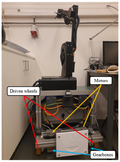
In this paper, we propose a motion control system for a low-cost differential drive mobile robot. The robotic platform is equipped with two driven wheels powered by Beckhoff motors, instrumented with incremental encoders. The control system is designed and implemented using Beckhoff's TwinCAT 3 automation software, running on an industrial PC. The system is tested and experimentally tuned to achieve optimal performance. The method allows addressing both odometry motion accuracy and motion correction in order to obtain minimum trajectory errors. Test results on linear and angular robot trajectories show errors below 0.02 and 0.03%, respectively, after tuning of the motion parameters. The proposed approach can be expanded, tweaked and applied to other differential drive TwinCAT 3 based robotic solutions. This will contribute to expanding mobile robot applications to a variety of fields, such as industrial automation, logistics, warehouse management, health care, ocean and space exploration and a variety of other industrial and non-industrial activities.

References

[1]	R. Siegwart, I. R. Nourbakhsh, Introduction to Autonomous Mobile Robots, Cambridge, Massachusetts: The MIT Press, 2004.
[2]	U. Nehmzow, Mobile robotics: A Practical Introduction, 2nd edition, Springer, (2012), 1–21.
[3]	F. Rubio, F. Valero, C. Llopis-Albert, A review of mobile robots: concepts, methods, theoretical framework, and applications, Int. J. Adv. Rob. Syst., 16 (2019). https://doi.org/10.1177/1729881419839 doi: 10.1177/1729881419839
[4]	L. Jaulin, Mobile Robotics, 2nd edition, London: ISTE Ltd; John Wiley & Sons, 2019. https://doi.org/10.1002/9781119663546
[5]	S. K. Malu, J. Majumdar, Kinematics, localization and control of differential drive mobile robot, Global J. Res. Eng., 14 (2014), 1–7. Available from: https://engineeringresearch.org/index.php/GJRE/article/view/1233.
[6]	G. Díaz-García, L. F. Giraldo, S. Jimenez-Leudo, Dynamics of a differential wheeled robot: control and trajectory error bound, in 2021 IEEE 5th Colombian Conference on Automatic Control (CCAC), (2021), 25–30. https://doi.org/10.1109/CCAC51819.2021.9633318
[7]	T. Hellström, Kinematics Equations for Differential Drive and Articulated Steering, Department of Computing Science, Umeå University, 2011. Available from: https://www.diva-portal.org/smash/get/diva2:796235/FULLTEXT01.pdf.
[8]	E. Maulana, M. A. Muslim, A. Zainuri, Inverse kinematics of a two-wheeled differential drive an autonomous mobile robot, in 2014 Electrical Power, Electronics, Communicatons, Control and Informatics Seminar (EECCIS), (2014), 93–98. https://doi.org/10.1109/EECCIS.2014.7003726
[9]	F. A. Salem, Dynamic and kinematic models and control for differential drive mobile robots, Int. J. Curr. Eng. Technol., 3 (2013), 253–263. Available from: https://inpressco.com/wp-content/uploads/2013/03/Paper6253-2632.pdf.
[10]	J. Borenstein, H. R. Everett, L. Feng, Where am I? Sensors and methods for mobile robot positioning, The University of Michigan, 1996. Available from: https://citeseerx.ist.psu.edu/document?repid=rep1&type=pdf&doi=80913ec26b835fd8238fe95c90c67770d528f9f9.
[11]	K. S. Chong, L. Kleeman, Accurate odometry and error modelling for a mobile robot, in Proceedings of International Conference on Robotics and Automation, 4 (1997), 2783–2788. https://doi.org/10.1109/ROBOT.1997.606708
[12]	J. Borenstein, L. Feng, Measurement and correction of systematic odometry errors in mobile robots, IEEE Trans. Rob. Autom., 12 (1996), 869–880. https://doi.org/10.1109/70.544770 doi: 10.1109/70.544770
[13]	R. B. Sousa, M. R. Petry, A. P. Moreira, Evolution of odometry calibration methods for ground mobile robots, in 2020 IEEE International Conference on Autonomous Robot Systems and Competitions (ICARSC), (2020), 294–299. https://doi.org/10.1109/ICARSC49921.2020.9096154
[14]	M. N. Zafar, J. C. Mohanta, Methodology for path planning and optimization of mobile robots: a review, Procedia Comput. Sci., 133 (2018), 141–152. https://doi.org/10.1016/j.procs.2018.07.018 doi: 10.1016/j.procs.2018.07.018
[15]	B. K. Patle, G. Babu L, A. Pandey, D. Parhi, A. Jagadeesh, A review: on path planning strategies for navigation of mobile robot, Def. Technol., 15 (2019), 582–606. https://doi.org/10.1016/j.dt.2019.04.011 doi: 10.1016/j.dt.2019.04.011
[16]	Q. B. Zhang, P. Wang, Z. H. Chen, An improved particle filter for mobile robot localization based on particle swarm optimization, Expert Syst. Appl., 135 (2019), 181–193. https://doi.org/10.1016/j.eswa.2019.06.006 doi: 10.1016/j.eswa.2019.06.006
[17]	W. Deng, J. Xu, X. Z. Gao, H. Zhao, An enhanced MSIQDE algorithm with novel multiple strategies for global optimization problems, IEEE Trans. Syst. Man Cybern.: Syst., 52 (2022), 1578–1587. https://doi.org/10.1109/TSMC.2020.3030792 doi: 10.1109/TSMC.2020.3030792
[18]	Y. Song, X. Cai, X. Zhou, B. Zhang, H. Chen, Y. Li, et al., Dynamic hybrid mechanism-based differential evolution algorithm and its application, Expert Syst. Appl., 213 (2023), 118834. https://doi.org/10.1016/j.eswa.2022.118834 doi: 10.1016/j.eswa.2022.118834
[19]	W. Deng, J. Xu, H. Zhao, Y. Song, A novel gate resource allocation method using improved PSO-based QEA, IEEE Trans. Intell. Transp. Syst., 23 (2022), 1737–1745. https://doi.org/10.1109/TITS.2020.3025796 doi: 10.1109/TITS.2020.3025796
[20]	W. Deng, X. Zhang, Y. Zhou, Y. Liu, X. Zhou, H. Chen, et al, An enhanced fast non-dominated solution sorting genetic algorithm for multi-objective problems, Inf. Sci., 585 (2022), 441–453. https://doi.org/10.1016/j.ins.2021.11.052 doi: 10.1016/j.ins.2021.11.052
[21]	H. Chen, F. Miao, Y. Chen, Y. Xiong, T. Chen, A hyperspectral image classification method using multifeature vectors and optimized KELM, IEEE J. Sel. Top. Appl. Earth Obs. Remote Sens., 14 (2021), 2781–2795. https://doi.org/10.1109/JSTARS.2021.3059451 doi: 10.1109/JSTARS.2021.3059451
[22]	Y. Yu, Z. Hao, G. Li, Y. Liu, R. Yang, H. Liu, Optimal search mapping among sensors in heterogeneous smart homes, Math. Biosci. Eng., 20 (2023), 1960–1980. https://doi.org/10.3934/mbe.2023090 doi: 10.3934/mbe.2023090
[23]	M. Aliff, N. Raihan, I. Yusof, N. Samsiah, Development of remote operated vehicle (ROV) control system using Twincat at main control pod (MCP), Int. J. Innovative Technol. Exploring Eng., 8 (2019), 12. https://doi.org/10.35940/ijitee.L4019.1081219 doi: 10.35940/ijitee.L1003.10812S219
[24]	L. Xie, C. Scheifele, W. Xu, K. A. Stol, Heavy-duty omni-directional Mecanum-wheeled robot for autonomous navigation: system development and simulation realization, in 2015 IEEE International Conference on Mechatronics (ICM), (2015), 256–261. https://doi.org/10.1109/ICMECH.2015.7083984
[25]	H. Liikanen, M. M. Aref, J. Mattila, M-Estimator application in real-time sensor fusion for smooth position feedback of heavy-duty field robots, in 2019 IEEE International Conference on Cybernetics and Intelligent Systems (CIS) and IEEE Conference on Robotics, Automation and Mechatronics (RAM), (2019), 368–373. https://doi.org/10.1109/CIS-RAM47153.2019.9095821
[26]	C. Scheifele, A. Lechler, C. Daniel, W. Xu, Real-time extension of ROS based on a network of modular blocks for highly precise motion generation, in 2016 IEEE 14th International Workshop on Advanced Motion Control (AMC), (2016), 129–134. https://doi.org/10.1109/AMC.2016.7496339
[27]	J. He, Y. Sun, L. Yang, J. Sun, Y. Xing, F. Gao, Design and control of TAWL—A wheel-legged rover with Terrain-adaptive wheel speed allocation capability, IEEE/ASME Trans. Mechatron., 27 (2022), 2212–2223. https://doi.org/10.1109/TMECH.2022.3176638 doi: 10.1109/TMECH.2022.3176638
[28]	L. Yu, D. Kong, X. Shao, X. Yan, A path planning and navigation control system design for driverless electric bus, IEEE Access, 6 (2018), 53960–53975. https://doi.org/10.1109/ACCESS.2018.2868339 doi: 10.1109/ACCESS.2018.2868339
[29]	T. da R. Anjo, Implementação e controlo de um robô móvel com braço antropomórfico, 2021. Available from: https://repositorio-aberto.up.pt/bitstream/10216/136886/2/507140.pdf.
[30]	W. Deng, H. Liu, J. Xu, H. Zhao, Y. Song, An improved quantum-inspired differential evolution algorithm for deep belief network, IEEE Trans. Instrum. Meas., 69 (2020), 7319–7327. https://doi.org/10.1109/TIM.2020.2983233 doi: 10.1109/TIM.2020.2983233
[31]	W. Deng, L. Zhang, X. Zhou, Y. Zhou, Y. Sun, W. Zhu, et al., Multi-strategy particle swarm and ant colony hybrid optimization for airport taxiway planning problem, Inf. Sci., 612 (2022), 576–593. https://doi.org/10.1016/j.ins.2022.08.115 doi: 10.1016/j.ins.2022.08.115

Reader Comments

Your name:*

Email:*
© 2023 the Author(s), licensee AIMS Press. This is an open access article distributed under the terms of the Creative Commons Attribution License (http://creativecommons.org/licenses/by/4.0)