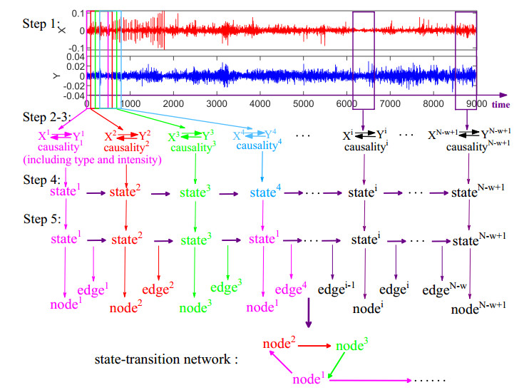
The causal inference method based on the time-series analysis has been subject to intense scrutiny, by which the interaction has been revealed between gold and the dollar. The positive or negative causality between them has been captured by the existing methods. However, the dynamic interactions are time-varying rather than immutable, i.e., the evolution of the causality between gold and the dollar is likely to be covered by the statistical process. In this article, a method which combines the pattern causality and the state-transition network is developed to identify the characteristics of the causality evolution between gold and the dollar. Based on this method, we can identify not only the causality intensity but also the causality type, including the types of positive causality, negative causality and the third causality (dark causality). Furthermore, the patterns of the causalities for the segments of the bivariate time series are transformed to a state-transition network from which the characteristics in the evolution of the causality have also been identified. The results show that the causality has some prominent motifs over time, that are the states of negative causality. More interestingly, the states that act as a bridge in the transition between states are also negative causality. Therefore, our findings provide a new perspective to explain the relatively stable negative causality between gold and the dollar from the evolution of causality. It can also help market participants understand and monitor the dynamic process of causality between gold and the dollar.
Citation: Ping Wang, Changgui Gu, Huijiu Yang, Haiying Wang. Identify the characteristic in the evolution of the causality between the gold and dollar[J]. Electronic Research Archive, 2022, 30(10): 3660-3678. doi: 10.3934/era.2022187
The causal inference method based on the time-series analysis has been subject to intense scrutiny, by which the interaction has been revealed between gold and the dollar. The positive or negative causality between them has been captured by the existing methods. However, the dynamic interactions are time-varying rather than immutable, i.e., the evolution of the causality between gold and the dollar is likely to be covered by the statistical process. In this article, a method which combines the pattern causality and the state-transition network is developed to identify the characteristics of the causality evolution between gold and the dollar. Based on this method, we can identify not only the causality intensity but also the causality type, including the types of positive causality, negative causality and the third causality (dark causality). Furthermore, the patterns of the causalities for the segments of the bivariate time series are transformed to a state-transition network from which the characteristics in the evolution of the causality have also been identified. The results show that the causality has some prominent motifs over time, that are the states of negative causality. More interestingly, the states that act as a bridge in the transition between states are also negative causality. Therefore, our findings provide a new perspective to explain the relatively stable negative causality between gold and the dollar from the evolution of causality. It can also help market participants understand and monitor the dynamic process of causality between gold and the dollar.

| [1] |
N. Apergis, Can gold prices forecast the Australian dollar movements? Int. Rev. Econ. Finance, 29 (2014), 75–82. http://doi.org/10.1016/j.iref.2013.04.004 doi: 10.1016/j.iref.2013.04.004

|
| [2] |
T. D. Kaufmann, R. A. Winters, The price of gold: a simple model, Resour. Policy 15 (1989), 309–313. https://doi.org/10.1016/0301-4207(89)90004-4 doi: 10.1016/0301-4207(89)90004-4
|
| [3] |
B. Mo, H. Nie, Y. Jiang, Dynamic linkages among the gold market, US dollar and crude oil market, Phys. A, 491 (2017), 984–994. https://doi.org/10.1016/j.physa.2017.09.091 doi: 10.1016/j.physa.2017.09.091
|
| [4] |
X. M. Ma, R. X. Yang, D. Zou, R. Liu, Measuring extreme risk of sustainable financial system using GJR-GARCH model trading data-based, Int. J. Inf. Manage., 50 (2020), 526–537. https://doi.org/10.1016/j.ijinfomgt.2018.12.013 doi: 10.1016/j.ijinfomgt.2018.12.013
|
| [5] |
Z. H. Ding, K. Shi, B. Wang, Dollar's influence on crude oil and gold based on MF-DPCCA method, Discrete Dyn. Nat. Soc., 2021 (2021), 5558967. https://doi.org/10.1155/2021/5558967 doi: 10.1155/2021/5558967
|
| [6] |
J. Chai, C. Y. Zhao, Y. Hu, Z. G. Zhang, Structural analysis and forecast of gold price returns, J. Manage. Sci. Eng., 6 (2021), 135–145. https://doi.org/10.1016/j.jmse.2021.02.011 doi: 10.1016/j.jmse.2021.02.011
|
| [7] |
N. Diniz-Maganini, E. H. Dinizb, A. A. Rasheedc, Bitcoin's price efficiency and safe haven properties during the COVID-19 pandemic: a comparison, Res. Int. Bus. Finance, 58 (2021), 101472. https://doi.org/10.1016/j.ribaf.2021.101472 doi: 10.1016/j.ribaf.2021.101472
|
| [8] |
R. W. Jastram, The Golden Constant, J. Econ., 100 (2010), 189–190. http://doi.org/10.1007/s00712-010-0124-5 doi: 10.1007/s00712-010-0124-5
|
| [9] |
B. M. Lucey, E. Tully, Seasonality, risk and return in daily comex gold and silver, Appl. Financ. Econ., 16 (2006), 319–333. http://doi.org/10.1080/09603100500386586 doi: 10.1080/09603100500386586
|
| [10] |
M. Joy, Gold and the US dollar: hedge or haven? Finance Res. Lett., 8 (2011), 120–131. http://doi.org/10.1016/j.frl.2011.01.001 doi: 10.1016/j.frl.2011.01.001
|
| [11] |
C. S. Liu, M. S. Chang, X. M. Wu, C. M. Chui, Hedges or safe havens–revisit the role of gold and USD against stock: a multivariate extended skew-t copula approach, Quant. Finance, 16 (2016), 1763–1789. http://doi.org/10.1080/14697688.2016.1176238 doi: 10.1080/14697688.2016.1176238
|
| [12] |
K. Pukthuanthong, R. Roll, Gold and the Dollar (and the Euro, Pound, and Yen), J. Banking Finance, 35 (2011), 2070–2083. http://doi.org/10.1016/j.jbankfin.2011.01.014 doi: 10.1016/j.jbankfin.2011.01.014
|
| [13] |
J. C. Reboredo, Is gold a safe haven or a hedge for the US dollar? Implications for risk management, J. Banking Finance, 37 (2013), 2665–2676. http://doi.org/10.1016/j.jbankfin.2013.03.020 doi: 10.1016/j.jbankfin.2013.03.020
|
| [14] |
F. Capie, T. C. Mills, G. Wood, Gold as a hedge against the dollar, J. Int. Financ. Mark., Inst. Money, 15 (2005), 343–352. http://doi.org/10.1016/j.intfin.2004.07.002 doi: 10.1016/j.intfin.2004.07.002
|
| [15] |
M. Massimiliano, Z. Paolo, Gold and the U.S. dollar: tales from the turmoil, Quant. Finance, 13 (2013), 571–582. http://doi.org/10.2139/ssrn.1598745 doi: 10.2139/ssrn.1598745
|
| [16] |
F. L. Lin, Y. F. Chen, S. Y. Yang, Does the value of US dollar matter with the price of oil and gold? A dynamic analysis from time-frequency space, Int. Rev. Econ. Finance, 43 (2016), 59–71. https://doi.org/10.1016/j.iref.2015.10.031 doi: 10.1016/j.iref.2015.10.031
|
| [17] |
H. An, X. Y. Gao, W. Fang, Y. Ding, W. Zhong, Research on patterns in the fluctuation of the co-movement between crude oil futures and spot prices: a complex network approach, Appl. Energy, 136 (2014), 1067–1075. https://doi.org/10.1016/j.apenergy.2014.07.081 doi: 10.1016/j.apenergy.2014.07.081
|
| [18] |
A. L. Barabasi, R. Albert, Emergence of scaling in random networks, Science, 286 (1999), 509–512. https://doi.org/10.1126/science.286.5439.509 doi: 10.1126/science.286.5439.509
|
| [19] |
M. E. J. Newman, D. J. Watts, Renormalization group analysis of the small-world network model, Phys. Lett., 263 (1999), 341–346. https://doi.org/10.1016/S0375-9601(99)00757-4 doi: 10.1016/S0375-9601(99)00757-4
|
| [20] |
L. Lacasa, B. Luque, F. J. Ballesteros, J. Luque, J. C. Nuno, From time series to complex networks: the visibility graph, Proc. Natl. Acad. Sci. U.S.A., 105 (2008), 4972–4975. http://doi.org/10.1073/pnas.0709247105 doi: 10.1073/pnas.0709247105
|
| [21] |
R. V. Donner, M. Small, J. F. Donges, N. Marwan, Y. Zou, R. Xiang, et al., Recurrence-based time series analysis by means of complex network methods, Int. J. Bifurcation Chaos, 21 (2011), 1019–1046. https://doi.org/10.1142/S0218127411029021 doi: 10.1142/S0218127411029021
|
| [22] |
X. Y. Gao, W. Fang, F. An, Y. Wang, Detecting method for crude oil price fluctuation mechanism under different periodic time series, Appl. Energy, 192 (2017), 201–212. https://doi.org/10.1016/j.apenergy.2017.02.014 doi: 10.1016/j.apenergy.2017.02.014
|
| [23] |
X. Han, Y. Zhao, M. Small, Identification of dynamical behavior of pseudoperiodic time series by network community structure, IEEE Trans. Circuits Syst. Ⅱ: Express Briefs, 66 (2019), 1905–1909. https://doi.org/10.1109/TCSII.2019.2903936 doi: 10.1109/TCSII.2019.2903936
|
| [24] |
Y. Zhao, T. Weng, S. Ye, Geometrical invariability of transformation between a time series and a complex network, Phys. Rev. E, 90 (2014), 012804. https://doi.org/10.1103/PhysRevE.90.012804 doi: 10.1103/PhysRevE.90.012804
|
| [25] |
C. Zhou, L. Ding, Y. Zhou, H. Luo, Topological mapping and assessment of multiple settlement time series in deep excavation: a complex network perspective, Adv. Eng. Inf., 36 (2018), 1–19. https://doi.org/10.1016/j.aei.2018.02.005 doi: 10.1016/j.aei.2018.02.005
|
| [26] |
S. Mutua, C. G. Gu, H. j. Yang, Visibility graphlet approach to chaotic time series, Chaos, 26 (2016), 053107. http://doi.org/10.1063/1.4951681 doi: 10.1063/1.4951681
|
| [27] |
Z. K. Gao, Q. Cai, Y. X. Yang, W. D. Dang, S. S. Zhang, Multiscale limited penetrable horizontal visibility graph for analyzing nonlinear timeseries, Sci. Rep., 6 (2016), 035622. https://doi.org/10.1038/srep35622 doi: 10.1038/srep35622
|
| [28] |
Y. Y. Zhao, C. G. Gu, H. J. Yang, Visibility-graphlet approach to the output series of a Hodgkin-Huxley neuron, Chaos, 31 (2021), 043102. https://doi.org/10.1063/5.0018359 doi: 10.1063/5.0018359
|
| [29] |
J. Zhang, D. C. Broadstock, The causality between energy consumption and economic growth for China in a time-varying framework, Energy J., 37 (2016), 29–53. https://doi.org/10.5547/01956574.37.SI1.jzha doi: 10.5547/01956574.37.SI1.jzha
|
| [30] |
O. Nataf, L. De Moor, Debt rating downgrades of financial institutions: causality tests on single-issue CDS and iTraxx, Quant. Finance, 19 (2019), 1975–1993. https://doi.org/10.1080/14697688.2019.1619933 doi: 10.1080/14697688.2019.1619933
|
| [31] |
T. Wu, X. Y. Gao, S. F. An, S. Y. Liu, Diverse causality inference in foreign exchange markets, Int. J. Bifurcation Chaos, 31 (2021), 2150070. https://doi.org/10.1142/S021812742150070X doi: 10.1142/S021812742150070X
|
| [32] |
G. Sugihara, Detecting causality in complex ecosystems, Science, 338 (2012), 496–500. https://doi.org/10.1126/science.1227079 doi: 10.1126/science.1227079
|
| [33] |
S. Y. Leng, H. F. Ma, J. Kurths, Y. C. Lai, W. Lin, K. Aihara, et al., Partial cross mapping eliminates indirect causal influences, Nat. Commun., 11 (2020), 2632. http://doi.org/10.1038/s41467-020-16238-0 doi: 10.1038/s41467-020-16238-0
|
| [34] |
S. K. Stavroglou, A. A. Pantelous, H. E. Stanley, K. M. Zuev, Hidden interactions in financial markets, Proc. Natl. Acad. Sci., 116 (2019), 10646–10651. http://doi.org/10.1073/pnas.1819449116 doi: 10.1073/pnas.1819449116
|
| [35] |
S. K. Stavroglou, A. A. Pantelous, H. E. Stanley, K. M. Zuev, Unveiling causal interactions in complex systems, Proc. Natl. Acad. Sci., 117 (2020), 7599–7605. http://doi.org/10.1073/pnas.1918269117 doi: 10.1073/pnas.1918269117
|
| [36] |
G. Sugihara, R. M. May, Nonlinear forecasting as a way of distinguishing chaos from measurement error in time series, Nature, 344 (1990), 734–741. http://doi.org/10.1038/344734a0 doi: 10.1038/344734a0
|
| [37] | F. Takens, Dynamical systems and turbulence, Lect. Notes Math., Springer-Verlag, New York, 898 (1981), 366–381. |
| [38] |
H. S. Kim, R. Eykholt, J. D. Salas, Nonlinear dynamics, delay times, and embedding windows, Phys. D, 127 (1999), 48–60. https://doi.org/10.1016/S0167-2789(98)00240-1 doi: 10.1016/S0167-2789(98)00240-1
|
| [39] |
R. Milo, S. Shen-Orr, S. Itzkovitz, N. Kashtan, D. Chklovskii, U. Alon, Network motifs: simple building blocks of complex networks, Science, 298 (2002), 824–827. https://doi.org/10.1126/science.298.5594.824 doi: 10.1126/science.298.5594.824
|
| [40] |
A. Reka, A. Barabasi, Statistical mechanics of complex networks, Rev. Mod. Phys., 74 (2002), 47–97. https://doi.org/10.1103/RevModPhys.74.47 doi: 10.1103/RevModPhys.74.47
|
| [41] |
M. S. Taqqu, V. Teverovsky, W. Willinger, Estimators for long-range dependence: an empirical study, Fractals, 3 (1995), 785–798. https://doi.org/10.1142/S0218348X95000692 doi: 10.1142/S0218348X95000692
|
| [42] |
H. E. Hurst, Long-term syorage capacity of reservoirs, Trans. Am. Soc. Civ. Eng., 116 (1951), 770–799. https://doi.org/10.1061/TACEAT.0006518 doi: 10.1061/TACEAT.0006518
|
| [43] | E. E. Peters, Fractal Market Analysis: Applying Chaos Theory to Investment and Economics, Inc: John Wiley Sons, 1994. Available from: https://vdoc.pub/documents/fractal-market-analysis-applying-chaos-theory-to-investment-and-economics-2eb6d1gv7jsg. |
| [44] | A. Barulescu, C. Serban, C. Maftel, Evaluation of Hurst exponent for precipitation time series, in Proceedings of the 14th WSEAS international conference on Computers: part of the 14th WSEAS CSCC multiconference, (2010), 590–595. Available from: https://www.researchgate.net/publication/262253543. |
| [45] |
P. M. Robinson, Gaussian semiparametric estimation of longrange dependence, Ann. Stat., 23 (1995), 1630–1661. https://doi.org/10.1214/aos/1176324317 doi: 10.1214/aos/1176324317
|
| [46] |
G. W. Wornell, A. V. Oppenheim, Estimation of fraetal signals from noisy measurements using wavelets, IEEE Trans. Signal Process., 40 (1992), 61l–623. https://doi.org/10.1109/78.120804 doi: 10.1109/78.120804
|
| [47] | S. Fortunato, C. Castellano, Community structure in graphs, Comput. Complexity, Springer, New York, preprint, arXiv: 0712.2716. |
| [48] |
X. T. Sun, W. Fang, X. Y. Gao, S. F. An, S. Y. Liu, T. Wu, Time-varying causality inference of different nickel markets based on the convergent cross mapping method, Resour. Policy, 74 (2021), 102385. https://doi.org/10.1016/j.resourpol.2021.102385 doi: 10.1016/j.resourpol.2021.102385
|
| [49] |
V. D. Blondel, J. L. Guillaume, R. Lambiotte, E. Lefebvre, Fast unfolding of communities in large networks, J. Stat. Mech.: Theory Exp., 10 (2008), P10008. https://doi.org/10.1088/1742-5468/2008/10/P10008 doi: 10.1088/1742-5468/2008/10/P10008
|


Figures(7) / Tables(1)
Ping Wang, Changgui Gu, Huijiu Yang, Haiying Wang. Identify the characteristic in the evolution of the causality between the gold and dollar[J]. Electronic Research Archive, 2022, 30(10): 3660-3678. doi: 10.3934/era.2022187


 DownLoad: