Wastewater treatment by microalgae is an eco-friendly and sustainable method for pollutant removal and biomass generation. Microalgae production under abiotic stress (such as salinity/salt stress) has an impact on nutrient removal and fatty acid accumulation. In this study, a freshwater microalgal strain (Desmodesmus communis GEEL-12) was cultured in municipal wastewater with various NaCl concentrations (ranging from 25–150 mM). The growth kinetics and morphological changes of the microalgae were observed. The nutrient removal, salinity change, fatty acid composition, and biodiesel quality under various groups were also investigated. The maximum growth of D. communis GEEL-12 was observed in the control group at 0.48 OD680nm. The growth inhibition was observed under high salt conditions (150 mM), which showed poor tolerance with 0.15 OD680nm. The nitrogen (N) and phosphorus (P) removal significantly decreased from 99–81% and 5.0–5.9% upon the addition of 100–150 mM salt, respectively. Palmitic acid (C16:0) and stearic acid (C18:0) were the most common fatty acid profiles. The abundance of C18:0 enhanced from 49.37%–56.87% in D. communis GEEL-12 upon high NaCl concentrations (100–150 mM). The biodiesel quality index of D. communis GEEL-12 under 50–75 mM salt concentrations reached the levels advised by international standards.
Citation: Adel I. Alalawy, Yang Yang, Fahad M. Almutairi, Haddad A. El Rabey, Mohammed A. Al-Duais, Abdelfatah Abomohra, El-Sayed Salama. Freshwater microalgae-based wastewater treatment under abiotic stress[J]. AIMS Environmental Science, 2023, 10(4): 504-515. doi: 10.3934/environsci.2023028
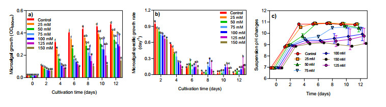
Wastewater treatment by microalgae is an eco-friendly and sustainable method for pollutant removal and biomass generation. Microalgae production under abiotic stress (such as salinity/salt stress) has an impact on nutrient removal and fatty acid accumulation. In this study, a freshwater microalgal strain (Desmodesmus communis GEEL-12) was cultured in municipal wastewater with various NaCl concentrations (ranging from 25–150 mM). The growth kinetics and morphological changes of the microalgae were observed. The nutrient removal, salinity change, fatty acid composition, and biodiesel quality under various groups were also investigated. The maximum growth of D. communis GEEL-12 was observed in the control group at 0.48 OD680nm. The growth inhibition was observed under high salt conditions (150 mM), which showed poor tolerance with 0.15 OD680nm. The nitrogen (N) and phosphorus (P) removal significantly decreased from 99–81% and 5.0–5.9% upon the addition of 100–150 mM salt, respectively. Palmitic acid (C16:0) and stearic acid (C18:0) were the most common fatty acid profiles. The abundance of C18:0 enhanced from 49.37%–56.87% in D. communis GEEL-12 upon high NaCl concentrations (100–150 mM). The biodiesel quality index of D. communis GEEL-12 under 50–75 mM salt concentrations reached the levels advised by international standards.

| [1] |
Liu X, Dai J, Wu D, et al. (2016) Sustainable application of a novel water cycle using seawater for toilet flushing. Engineering 2: 460–469. https://doi.org/10.1016/J.ENG.2016.04.013 doi: 10.1016/J.ENG.2016.04.013

|
| [2] |
Li C, Gao X, Li S, et al. (2020) A review of the distribution, sources, genesis, and environmental concerns of salinity in groundwater. Environ Sci Pollut Res 27: 41157–41174. https://doi.org/10.1007/s11356-020-10354-6 doi: 10.1007/s11356-020-10354-6
|
| [3] |
Ali S, Peter A P, Chew K W, et al. (2021) Resource recovery from industrial effluents through the cultivation of microalgae: A review. Bioresour Technol 337: 125461. https://doi.org/10.1016/j.biortech.2021.125461 doi: 10.1016/j.biortech.2021.125461
|
| [4] |
Shi J, Huang W, Han H, et al. (2020) Review on treatment technology of salt wastewater in coal chemical industry of China. Desalination 493. https://doi.org/10.1016/j.desal.2020.114640 doi: 10.1016/j.desal.2020.114640
|
| [5] |
Crini G, Lichtfouse E (2019) Advantages and disadvantages of techniques used for wastewater treatment. Environ Chem Lett 17: 145–155. https://doi.org/10.1007/s10311-018-0785-9 doi: 10.1007/s10311-018-0785-9
|
| [6] |
Zhao Y, Zhuang X, Ahmad S, et al. (2020) Biotreatment of high-salinity wastewater: current methods and future directions. World J Microbiol Biotechnol 36. https://doi.org/10.1007/s11274-020-02815-4 doi: 10.1007/s11274-020-02815-4
|
| [7] |
Pollice A, Rozzi A, Tomei M C, et al. (2000) Monitoring the Inhibitory Effect of NaCl on Anaerobic Wastewater Treatment Processes by the Rantox Biosensor. Environ Technol 21: 535–544. https://doi.org/10.1080/09593332408618095 doi: 10.1080/09593332408618095
|
| [8] |
Zhang Y, Kuroda M, Arai S, et al. (2019) Biological treatment of selenate-containing saline wastewater by activated sludge under oxygen-limiting conditions. Water Res 154: 327–335. https://doi.org/10.1016/j.watres.2019.01.059 doi: 10.1016/j.watres.2019.01.059
|
| [9] |
Sun C, Xia A, Liao Q, et al. (2019) Life-cycle assessment of biohythane production via two-stage anaerobic fermentation from microalgae and food waste. Renewe Sust Energ Rev 112: 395–410. https://doi.org/10.1016/j.rser.2019.05.061 doi: 10.1016/j.rser.2019.05.061
|
| [10] |
Arif M, Li Y, El-Dalatony M M, et al. (2021) A complete characterization of microalgal biomass through FTIR/TGA/CHNS analysis: An approach for biofuel generation and nutrients removal. Renew Energy 163: 1973–1982. https://doi.org/10.1016/j.renene.2020.10.066 doi: 10.1016/j.renene.2020.10.066
|
| [11] |
Li X, Yuan Y, Cheng D, et al. (2018) Exploring stress tolerance mechanism of evolved freshwater strain Chlorella sp S30 under 30 g/L salt. Bioresource Technol 250: 495–504. https://doi.org/10.1016/j.biortech.2017.11.072 doi: 10.1016/j.biortech.2017.11.072
|
| [12] |
Srivastava G, Goud V V (2017) Salinity induced lipid production in microalgae and cluster analysis (ICCB 16-BR_047). Bioresource Technol 242: 244–252. https://doi.org/10.1016/j.biortech.2017.03.175 doi: 10.1016/j.biortech.2017.03.175
|
| [13] |
Paliwal C, Mitra M, Bhayani K, et al. (2017) Abiotic stresses as tools for metabolites in microalgae. Bioresource Technol 244: 1216–1226. https://doi.org/10.1016/j.biortech.2017.05.058 doi: 10.1016/j.biortech.2017.05.058
|
| [14] |
Darvehei P, Bahri P A, Moheimani N R. (2018) Model development for the growth of microalgae: A review. Renew Sust Energ Rev 97: 233–258. https://doi.org/10.1016/j.rser.2018.08.027 doi: 10.1016/j.rser.2018.08.027
|
| [15] |
Kashyap S P, Prasanna H C, Kumari N, et al. (2020) Understanding salt tolerance mechanism using transcriptome profiling and de novo assembly of wild tomato Solanum chilense. Sci Rep 10: 15835. https://doi.org/10.1038/s41598-020-72474-w doi: 10.1038/s41598-020-72474-w
|
| [16] |
Zhang M, Jalalah M, Alsareii S A, et al. (2023) Growth kinetics and metabolic characteristics of five freshwater indigenous microalgae for nutrient removal and biofuel generation: a sustainable approach. Biomass Convers Bior. https://doi.org/10.1007/s13399-023-03771-3 doi: 10.1007/s13399-023-03771-3
|
| [17] |
Bligh E G, Dyer W J (1959) A rapid method of total lipid extraction and purification. Can J Biochem Phys 37: 911–7. https://doi.org/10.1139/y59-099 doi: 10.1139/y59-099
|
| [18] |
Lepage G, Roy C C (1984) Improved recovery of fatty-acid through direct trans-esterification without prior extraction or purification. J Lipid Res 25: 1391–1396. https://doi.org/10.1016/S0022-2275(20)34457-6 doi: 10.1016/S0022-2275(20)34457-6
|
| [19] |
Katiyar R, Bharti R K, Gurjar B R, et al. (2018) Utilization of de-oiled algal biomass for enhancing vehicular quality biodiesel production from Chlorella sp in mixotrophic cultivation systems. Renew Energy 122: 80–88. https://doi.org/10.1016/j.renene.2018.01.037 doi: 10.1016/j.renene.2018.01.037
|
| [20] |
Abomohra A E F, El-Naggar A H, Baeshen A A (2018) Baeshen, Potential of macroalgae for biodiesel production: Screening and evaluation studies. J Biosci Bioeng 125: 231–237. https://doi.org/10.1016/j.jbiosc.2017.08.020 doi: 10.1016/j.jbiosc.2017.08.020
|
| [21] |
Rismani S, Shariati M (2017) Changes of the Total Lipid and Omega-3 Fatty Acid Contents in two Microalgae Dunaliella Salina and Chlorella Vulgaris Under Salt Stress. Braz Arch Biol Techn 60: e17160555–e17160555. https://doi.org/10.1590/1678-4324-2017160555 doi: 10.1590/1678-4324-2017160555
|
| [22] |
Gatamaneni B L, Orsat V, Lefsrud M (2018) Factors Affecting Growth of Various Microalgal Species. Environ Eng Sci 35: 1037–1048. https://doi.org/10.1089/ees.2017.0521 doi: 10.1089/ees.2017.0521
|
| [23] |
Arora N, Kumari P, Kumar A, et al. (2019) Delineating the molecular responses of a halotolerant microalga using integrated omics approach to identify genetic engineering targets for enhanced TAG production. Biotechnol Biofuels 12. https://doi.org/10.1186/s13068-018-1343-1 doi: 10.1186/s13068-018-1343-1
|
| [24] |
Rai M P, Gautom T, Sharma N (2015) Effect of Salinity, pH, Light Intensity on Growth and Lipid Production of Microalgae for Bioenergy Application. OnLine J Biol Sci 15. https://doi.org/10.3844/ojbsci.2015.260.267 doi: 10.3844/ojbsci.2015.260.267
|
| [25] |
Zhu C, Zhai X, Xi Y, et al. (2020) Efficient CO2 capture from the air for high microalgal biomass production by a bicarbonate Pool. J Co2 Util 37: 320–327. https://doi.org/10.1016/j.jcou.2019.12.023 doi: 10.1016/j.jcou.2019.12.023
|
| [26] |
Yang Q, Zhang M, Alwathnani H A, et al. (2022) Cultivation of Freshwater Microalgae in Wastewater Under High Salinity for Biomass, Nutrients Removal, and Fatty Acids/Biodiesel Production. Waste Biomass Valor 13: 3245–3254. https://doi.org/10.1007/s12649-022-01712-1 doi: 10.1007/s12649-022-01712-1
|
| [27] |
Vo H N P, Ngo H H, Guo W, et al. (2019) Identification of the pollutants' removal and mechanism by microalgae in saline wastewater. Bioresource Technol 275: 44–52. https://doi.org/10.1016/j.biortech.2018.12.026 doi: 10.1016/j.biortech.2018.12.026
|
| [28] |
Figler A, B-Béres V, Dobronoki D, et al. (2019) Salt Tolerance and Desalination Abilities of Nine Common Green Microalgae Isolates. Water 11. https://doi.org/10.3390/w11122527 doi: 10.3390/w11122527
|
| [29] |
Figler A, B-Béres V, Dobronoki D, et al. (2021) Salinity-induced microalgal-based mariculture wastewater treatment combined with biodiesel production. Bioresource Technol 340. https://doi.org/10.1016/j.biortech.2021.125638 doi: 10.1016/j.biortech.2021.125638
|
| [30] |
Alketife A M, Judd S, Znad H (2017) Synergistic effects and optimization of nitrogen and phosphorus concentrations on the growth and nutrient uptake of a freshwater Chlorella vulgaris. Environ Technol 38: 94–102. https://doi.org/10.1080/09593330.2016.1186227 doi: 10.1080/09593330.2016.1186227
|
| [31] |
Ferreira G F, Rios Pinto L F, Carvalho P O, et al. (2021) Biomass and lipid characterization of microalgae genera Botryococcus, Chlorella, and Desmodesmus aiming high-value fatty acid production. Biomass Convers Bior 11: 1675–1689. https://doi.org/10.1007/s13399-019-00566-3 doi: 10.1007/s13399-019-00566-3
|
| [32] |
Fan J. (2017) Acclimation to NaCl and light stress of heterotrophic Chlamydomonas reinhardtii for lipid accumulation. J Biosci Bioeng 124: 302–308. https://doi.org/10.1016/j.jbiosc.2017.04.009 doi: 10.1016/j.jbiosc.2017.04.009
|
| [33] |
Shetty P, Gitau M M, Maróti G (2019) Salinity Stress Responses and Adaptation Mechanisms in Eukaryotic Green Microalgae. Cells 8. https://doi.org/10.3390/cells8121657 doi: 10.3390/cells8121657
|
| [34] |
Khona D K, Shirolikar S M, Gawde K K, et al. (2016) Characterization of salt stress-induced palmelloids in the green alga, Chlamydomonas reinhardtii. Algal Res 16: 434–448. https://doi.org/10.1016/j.algal.2016.03.035 doi: 10.1016/j.algal.2016.03.035
|
| [35] |
Neelam S, Subramanyam R (2013) Alteration of photochemistry and protein degradation of photosystem II from Chlamydomonas reinhardtii under high salt grown cells. J Photoch Photobio B 124: 63–70. https://doi.org/10.1016/j.jphotobiol.2013.04.007 doi: 10.1016/j.jphotobiol.2013.04.007
|
| [36] |
Ashour M, Elshobary M E, El-Shenody R, et al. (2019) Evaluation of a native oleaginous marine microalga Nannochloropsis oceanicafor dual use in biodiesel production and aquaculture feed. Biomass Bioenergy 120: 439–447. https://doi.org/10.1016/j.biombioe.2018.12.009 doi: 10.1016/j.biombioe.2018.12.009
|
| [37] |
Poh Z L, Kadir W N A, Lam M K, et al. (2020) The effect of stress environment towards lipid accumulation in microalgae after harvesting. Renew Energy 154: 1083–1091. https://doi.org/10.1016/j.renene.2020.03.081 doi: 10.1016/j.renene.2020.03.081
|
| [38] |
Li S, Li X, Ho S H (2022) Microalgae as a solution of third world energy crisis for biofuels production from wastewater toward carbon neutrality: An updated review. Chemosphere 291: 132863. https://doi.org/10.1016/j.chemosphere.2021.132863 doi: 10.1016/j.chemosphere.2021.132863
|
| [39] |
Srinuanpan S, Cheirsilp B, Prasertsan P, et al. (2018) Strategies to increase the potential use of oleaginous microalgae as biodiesel feedstocks: Nutrient starvations and cost-effective harvesting process. Renew Energy 122: 507–516. https://doi.org/10.1016/j.renene.2018.01.121 doi: 10.1016/j.renene.2018.01.121
|
| [40] | ASTM D (2018) Standard specification for biodiesel fuel blend stock (B100) for middle distillate fuels. ASTM International 6571–6508. |
| [41] |
Altun Ş (2014) Effect of the degree of unsaturation of biodiesel fuels on the exhaust emissions of a diesel power generator. Fuel 117: 450–457. https://doi.org/10.1016/j.fuel.2013.09.028 doi: 10.1016/j.fuel.2013.09.028
|
| [42] |
Ahmad S, Kothari R, Pathania D, et al. (2020) Optimization of nutrients from wastewater using RSMfor augmentation of Chlorella pyrenoidosa with enhanced lipid productivity, FAME content, and its quality assessment using fuel quality index. Biomass Convers Bior 10: 495–512. https://doi.org/10.1007/s13399-019-00443-z doi: 10.1007/s13399-019-00443-z
|
| [43] |
Yaşar F, Altun Ş (2018) Biodiesel properties of microalgae (Chlorella protothecoides) oil for use in diesel engines. Int J Green Energy 15: 941–946. https://doi.org/10.1080/15435075.2018.1529589 doi: 10.1080/15435075.2018.1529589
|


Figures(4)

Adel I. Alalawy, Yang Yang, Fahad M. Almutairi, Haddad A. El Rabey, Mohammed A. Al-Duais, Abdelfatah Abomohra, El-Sayed Salama. Freshwater microalgae-based wastewater treatment under abiotic stress[J]. AIMS Environmental Science, 2023, 10(4): 504-515. doi: 10.3934/environsci.2023028


 DownLoad: