Atmospheric dispersion modelling of gaseous emissions from Beirutinternational airport activities

Tharwat Mokalled; Stéphane Le Calvé; Nada Badaro-Saliba; Maher Abboud; Rita Zaarour; Wehbeh Farah; Jocelyne Adjizian-Gérard; Tharwat Mokalled; Stéphane Le Calvé; Nada Badaro-Saliba; Maher Abboud; Rita Zaarour; Wehbeh Farah; Jocelyne Adjizian-Gérard

doi:10.3934/environsci.2022033

AIMS Environmental Science

2022, Volume 9, Issue 5: 553-572. doi: 10.3934/environsci.2022033

Previous Article Next Article

Research article

Atmospheric dispersion modelling of gaseous emissions from Beirutinternational airport activities

1.
Environmental Research Center, Eastern Mediterranean Area (CREEMO), Geography Department, Saint Joseph University, Beirut 1104 2020, Lebanon
2.
Group of Atmospheric Physical Chemistry, the Institute of Chemistry and Processes for Energy, Environment and Health (ICPEES, UMR 7515, CNRS/University of Strasbourg), Strasbourg 67087, France
3.
Unité de recherche Environnement, Génomique et Protéomique (UR-EGP), Faculté des sciences, Université Saint-Joseph, Beirut 1107 2050, Lebanon

Received: 21 February 2022 Revised: 09 July 2022 Accepted: 27 July 2022 Published: 01 September 2022

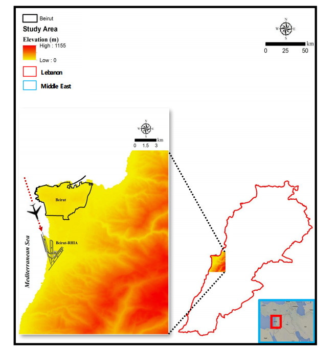
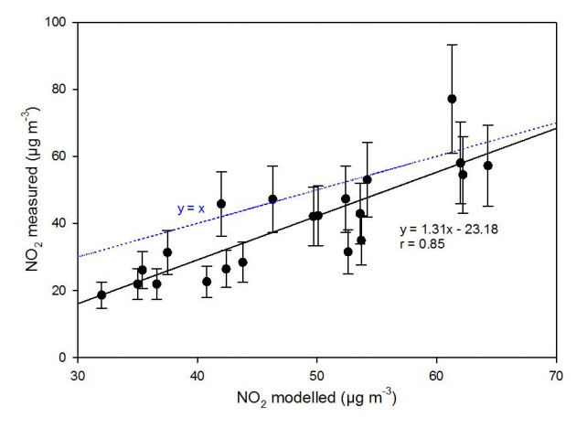
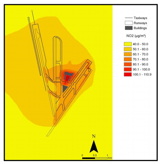
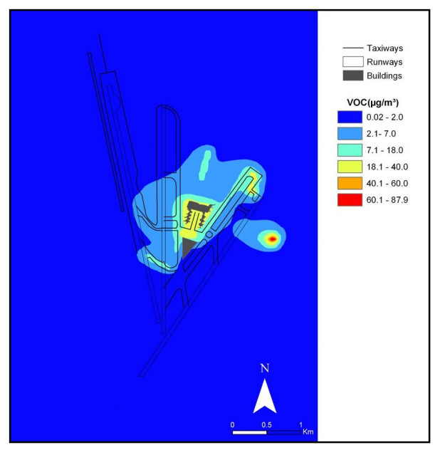
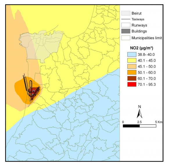
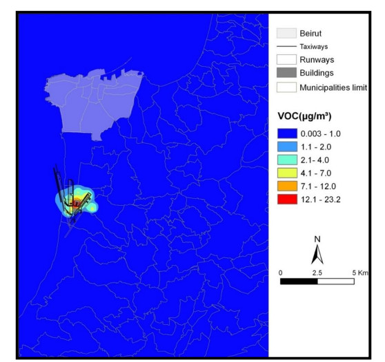
The projected increase of civil aviation activity, the degradation of air quality and the location of Beirut Airport embedded in a very urbanized area, in addition to the special geography and topography surrounding the airport which plays a significant role in drawing emissions to larger distances, demanded anassessment of the spatial impact of the airport activities on the air quality of Beirut and its suburbs. This is the first study in the Middle East region that model pollutant concentrations resulting from an international airport's activities using an advanced atmospheric dispersion modelling system in a country with no data. This followed validation campaigns showing very strong correlations (r = 0.85) at validation sites as close as possible to emission sources. The modelling results showed extremely high NO₂ concentrations within the airport vicinity, i.e., up to 110 μg∙m^-3 (which is greater than the World Health Organization annual guidelines) posing a health hazard to the workers in the ramp. The major contribution of Beirut–Rafic Hariri International Airport to the degradation of air quality was in the airport vicinity; however, it extended to Beirut and its suburbs in addition to affecting the seashore area due to emissions along the aircraft trajectory; this isan aspect rarely considered in previous studies. On the other hand, elevated volatile organic compound levels were observed near the fuel tanks and at the aerodrome center. This study provides (ⅰ) a methodology to assess pollutant concentrations resulting from airport emissions through the use of an advanced dispersion model in a country with no data; and (ⅱ) a tool for policy makers to better understand the contribution of the airport's operations to national pollutant emissions, which is vital for mitigation strategies and health impact assessments.
- aviation emission,
- atmospheric dispersion modelling system (ADMS),
- nitrogen dioxide,
- volatile organic compound,
- Beirut
Citation: Tharwat Mokalled, Stéphane Le Calvé, Nada Badaro-Saliba, Maher Abboud, Rita Zaarour, Wehbeh Farah, Jocelyne Adjizian-Gérard. Atmospheric dispersion modelling of gaseous emissions from Beirutinternational airport activities[J]. AIMS Environmental Science, 2022, 9(5): 553-572. doi: 10.3934/environsci.2022033

Related Papers:

Abstract

The projected increase of civil aviation activity, the degradation of air quality and the location of Beirut Airport embedded in a very urbanized area, in addition to the special geography and topography surrounding the airport which plays a significant role in drawing emissions to larger distances, demanded anassessment of the spatial impact of the airport activities on the air quality of Beirut and its suburbs. This is the first study in the Middle East region that model pollutant concentrations resulting from an international airport's activities using an advanced atmospheric dispersion modelling system in a country with no data. This followed validation campaigns showing very strong correlations (r = 0.85) at validation sites as close as possible to emission sources. The modelling results showed extremely high NO₂ concentrations within the airport vicinity, i.e., up to 110 μg∙m^-3 (which is greater than the World Health Organization annual guidelines) posing a health hazard to the workers in the ramp. The major contribution of Beirut–Rafic Hariri International Airport to the degradation of air quality was in the airport vicinity; however, it extended to Beirut and its suburbs in addition to affecting the seashore area due to emissions along the aircraft trajectory; this isan aspect rarely considered in previous studies. On the other hand, elevated volatile organic compound levels were observed near the fuel tanks and at the aerodrome center. This study provides (ⅰ) a methodology to assess pollutant concentrations resulting from airport emissions through the use of an advanced dispersion model in a country with no data; and (ⅱ) a tool for policy makers to better understand the contribution of the airport's operations to national pollutant emissions, which is vital for mitigation strategies and health impact assessments.

References

[1]	ICAO (2019) Aviation Benefits Report, Montreal, Global aviation Industry High-level Group. Available from https://www.icao.int/sustainability/Documents/AVIATION-BENEFITS-2019-web.pdf.
[2]	CAEP 9 (2013) Doc 10012, Committee on Aviation Environmental Protection, Ninth Meeting, 999 University Street, Montréal, Quebec, Canada H3C 5H7, ICAO 10012 CAEP.
[3]	Brasseur GP, Gupta M, Anderson BE, et al. (2015) Impact of Aviation on Climate: FAA's Aviation Climate Change Research Initiative (ACCRI) Phase Ⅱ. Bull Am Meteorol Soc.
[4]	FAA (2015) Aviation Emissions, Impacts & Mitigation A Primer, Office of Environment and Energy.
[5]	Mahashabde A, Wolfe P, Ashok A, et al. (2011) Assessing the environmental impacts of aircraft noise and emissions. Prog Aerosp Sci 47: 15–52. https://doi.org/10.1016/j.paerosci.2010.04.003 doi: 10.1016/j.paerosci.2010.04.003
[6]	Bendtsen KM, Bengtsen E, Saber AT, et al. (2021) A review of health effects associated with exposure to jet engine emissions in and around airports. Environ Health 20: 10. https://doi.org/10.1186/s12940-020-00690-y doi: 10.1186/s12940-020-00690-y
[7]	Jung K-H, Artigas F, Shin JY (2011) Personal, indoor, and outdoor exposure to VOCs in the immediate vicinity of a local airport. Environ Monit Assess 173: 555–567. https://doi.org/10.1007/s10661-010-1404-9 doi: 10.1007/s10661-010-1404-9
[8]	Levy JI, Woody M, Baek BH, et al. (2012) Current and future particulate-matter-related mortality risks in the United States from aviation emissions during landing and takeoff. Risk Anal Off Publ Soc Risk Anal 32: 237–249. https://doi.org/10.1111/j.1539-6924.2011.01660.x doi: 10.1111/j.1539-6924.2011.01660.x
[9]	Schindler BK, Weiss T, Schütze A, et al. (2013) Occupational exposure of air crews to tricresyl phosphate isomers and organophosphate flame retardants after fume events. Arch Toxicol 87: 645–648. https://doi.org/10.1007/s00204-012-0978-0 doi: 10.1007/s00204-012-0978-0
[10]	Yim SHL, Stettler MEJ, Barrett SRH (2013) Air quality and public health impacts of UK airports. Part Ⅱ: Impacts and policy assessment. Atmos Environ 67: 184–192. https://doi.org/10.1016/j.atmosenv.2012.10.017 doi: 10.1016/j.atmosenv.2012.10.017
[11]	Yim SHL, Lee GL, Lee IH, et al. (2015) Global, regional and local health impacts of civil aviation emissions. Environ Res Lett 10: 034001. https://doi.org/10.1088/1748-9326/10/3/034001 doi: 10.1088/1748-9326/10/3/034001
[12]	Kim BY (2012) Guidance for Quantifying the Contribution of Airport Emissions to Local Air Quality, Transportation Research Board. https://doi.org/10.17226/22757
[13]	Kim BY (2015) Understanding Airport Air Quality and Public Health Studies Related to Airports, Transportation Research Board. https://doi.org/10.17226/22119
[14]	Wood E (2008) Aircraft and Airport-related Hazardous Air Pollutants: Research Needs and Analysis, Transportation Research Board.
[15]	RIDEM (2008) Characterization of Ambient Air Toxics in Neighborhoods Abutting T.F. Green Airport and Comparison Sites: Final Report, Rhode Island Department of Environmental Management.
[16]	Zhu Y, Fanning E, Yu RC, et al. (2011) Aircraft emissions and local air quality impacts from takeoff activities at a large International Airport. Atmos Environ 45: 6526–6533. https://doi.org/10.1016/j.atmosenv.2011.08.062 doi: 10.1016/j.atmosenv.2011.08.062
[17]	Carslaw DC, Beevers SD, Ropkins K, et al. (2006) Detecting and quantifying aircraft and other on-airport contributions to ambient nitrogen oxides in the vicinity of a large international airport. Atmos Environ 40: 5424–5434. https://doi.org/10.1016/j.atmosenv.2006.04.062 doi: 10.1016/j.atmosenv.2006.04.062
[18]	Peace H, Maughan J, Owen B, et al. (2006) Identifying the contribution of different airport related sources to local urban air quality. Environ Model Softw 21: 532–538. https://doi.org/10.1016/j.envsoft.2004.07.014 doi: 10.1016/j.envsoft.2004.07.014
[19]	Farias F, ApSimon H (2006) Relative contributions from traffic and aircraft NOx emissions to exposure in West London. Environ Model Softw 21: 477–485. https://doi.org/10.1016/j.envsoft.2004.07.010 doi: 10.1016/j.envsoft.2004.07.010
[20]	Westerdahl D, Fruin SA, Fine PL, et al. (2008) The Los Angeles International Airport as a source of ultrafine particles and other pollutants to nearby communities. Atmos Environ 42: 3143–3155. https://doi.org/10.1016/j.atmosenv.2007.09.006 doi: 10.1016/j.atmosenv.2007.09.006
[21]	Koulidis AG, Progiou AG, Ziomas IC (2020) Air Quality Levels in the Vicinity of Three Major Greek Airports. Environ Model Assess 25: 749–760. https://doi.org/10.1007/s10666-020-09699-6 doi: 10.1007/s10666-020-09699-6
[22]	Hudda N, Gould T, Hartin K, et al. (2014) Emissions from an International Airport Increase Particle Number Concentrations 4-fold at 10 km Downwind. Environ Sci Technol 48: 6628–6635. https://doi.org/10.1021/es5001566 doi: 10.1021/es5001566
[23]	Mokalled T, Le Calvé S, Badaro-Saliba N, et al. (2018) Identifying the impact of Beirut Airport's activities on local air quality - Part Ⅰ: Emissions inventory of NO2 and VOCs. Atmos Environ 187: 435–444. https://doi.org/10.1016/j.atmosenv.2018.04.036 doi: 10.1016/j.atmosenv.2018.04.036
[24]	CERC (2015) EMIT: Atmospheric Emissions Inventory Toolkit User Guide. Version 3.4, 3 King's Parade. Carmbridge CB2 1SJ, Cambridge Environmental Research Consultant Ltd.
[25]	Mokalled T, Adjizian Gérard J, Abboud M, et al. (2019) An assessment of indoor air quality in the maintenance room at Beirut-Rafic Hariri International Airport. Atmospheric Pollut Res 10: 701–711. https://doi.org/10.1016/j.apr.2018.11.008 doi: 10.1016/j.apr.2018.11.008
[26]	Mokalled T, Adjizian Gérard J, Abboud M, et al. (2021) An Assessment of Indoor Air Quality in the Arrivals Hall of Beirut–Rafic Hariri International Airport: Monitoring of VOCs and NO2. Atmosphere 12: 400. https://doi.org/10.3390/atmos12030400 doi: 10.3390/atmos12030400
[27]	Baayoun A, Itani W, El Helou J, et al. (2019) Emission inventory of key sources of air pollution in Lebanon. Atmos Environ 215: 116871. https://doi.org/10.1016/j.atmosenv.2019.116871 doi: 10.1016/j.atmosenv.2019.116871
[28]	Salameh T, Afif C, Sauvage S, et al. (2014) Speciation of non-methane hydrocarbons (NMHCs) from anthropogenic sources in Beirut, Lebanon. Environ Sci Pollut Res 21: 10867–10877. https://doi.org/10.1007/s11356-014-2978-5 doi: 10.1007/s11356-014-2978-5
[29]	Waked A, Afif C (2012) Emissions of air pollutants from road transport in Lebanon and other countries in the Middle East region. Atmos Environ 61: 446–452. https://doi.org/10.1016/j.atmosenv.2012.07.064 doi: 10.1016/j.atmosenv.2012.07.064
[30]	Mokalled T, Adjizian Gérard J, Abboud M, et al. (2018) VOC tracers from aircraft activities at Beirut Rafic Hariri International Airport. Atmospheric Pollut Res. https://doi.org/10.1016/j.apr.2018.09.009 doi: 10.1016/j.apr.2018.09.009
[31]	ICAO (2008) Report of the independent experts on the LTTG NOx review and medium and long term technology goals for NOx., Montréal :, International Civil Aviation Organization.
[32]	Badaro-Saliba N, Adjizian-Gerard J, Zaarour R, et al. (2013) A geostatistical approach for assessing population exposure to NO2 in a complex urban area (Beirut, Lebanon). Stoch Environ Res Risk Assess 28: 467–474. https://doi.org/10.1007/s00477-013-0765-3 doi: 10.1007/s00477-013-0765-3
[33]	US EPA O (2021) US EPA, Volatile Organic Compounds' Impact on Indoor Air Quality, 2021. Available from: https://www.epa.gov/indoor-air-quality-iaq/volatile-organic-compounds-impact-indoor-air-quality.
[34]	Lebanese DGCA (2015) Statistics Department Daily Transactions.
[35]	Lebanese DGCA (2016) Statistics - Beirut Rafic Hariri International Airport, 2016. Available from: https://www.beirutairport.gov.lb/_statistic.php.
[36]	Lebanese DGCA (2017) eAIS Package for Lebanon, 2017. Available from: https://eaip.austrocontrol.at/all/ol/170105/2017-01-05-AIRAC/index.html.
[37]	CERC (2017) ADMS-AIrport User Guide. version 4.1.1, 3 King's Parade. Carmbridge CB2 1SJ, Cambridge Environmental Research Consultant Ltd.
[38]	CERC (2021) CERC > Environmental software > ADMS-Airport > Input and output, 2021. Available from: https://www.cerc.co.uk/environmental-software/ADMS-Airport-model/data.html.
[39]	ICAO (2011) Airport Air Quality Manual (Doc 9889).
[40]	Azzi M, Johnson (1992) An introduction to the generic reaction set photochemical smog mechanism, Proc. 11th Clean Air Conference, Brisbane, Australia, Best, P., Bofinger, N. and Cliff, D., 451–462.
[41]	Venkatram A, Karamchandani P, Pai P, et al. (1994) The development and application of a simplified ozone modeling system (SOMS). Atmos Environ 28: 3665–3678. https://doi.org/10.1016/1352-2310(94)00190-V doi: 10.1016/1352-2310(94)00190-V
[42]	Carruthers DJ, McHugh C, Jackson M, et al. (2011) Developments in ADMS-Airport to take account of near field dispersion and applications to Heathrow Airport. Int J Environ Pollut 44: 332. https://doi.org/10.1504/IJEP.2011.038434 doi: 10.1504/IJEP.2011.038434
[43]	CAEP (2008) LAQ Candidate Models Capabilities and Inter-Comparison Study.
[44]	CERC (2021) CERC > Environmental software > ADMS-Airport model, 2021. Available from: https://www.cerc.co.uk/environmental-software/ADMS-Airport-model.html.
[45]	DfT (2006) Project for the Sustainable Development of Heathow - Report of the Air Quality Technical Panels.
[46]	McHugh C (2007) Air Quality Studies for Heathrow: Base Case, Segregated Mode, Mixed Mode and Third Runway Scenarios modelled using ADMS-Airport.
[47]	CERC (2022) CERC > Environmental software > ADMS-Airport > Model options, 2022. Available from: https://www.cerc.co.uk/environmental-software/ADMS-Airport-model/options.html.
[48]	FAA (2014) Aviation Emissions and Air Quality Handbook Version 3.
[49]	Saltzman BE (1954) Colorimetric Microdetermination of Nitrogen Dioxide in Atmosphere. Anal Chem 26: 1949–1955. https://doi.org/10.1021/ac60096a025 doi: 10.1021/ac60096a025
[50]	Glasius M, Funch Carlsen M, Stroyer Hansen T, et al. (1999) Measurements of nitrogen dioxide on Funen using diffusion tubes. Atmos Environ 33: 1177–1185. https://doi.org/10.1016/S1352-2310(98)00285-4 doi: 10.1016/S1352-2310(98)00285-4
[51]	Passam (2017) Nitrogen Dioxide – passam, 2017. Available from: http://www.passam.ch/wp/nitrogen-dioxide/.
[52]	Carruthers DJ, McHugh C, Church S, et al. (2008) ADMS-AIRPORT: MODEL INTER-COMPARISIONS AND MODEL VALIDATION, CERC, 3 King's Parade, Cambridge CB2 1SJ, UK.
[53]	Carruthers DJ, Gray S, Johnson K, et al. (2007) Intercomparison of five modelling approaches including ADMS-Airport and EDMS/AERMOD for predicting air quality in the vicinity of London Heathrow Airport, Air and Waste Management Association—Guideline on Air Quality Models: Applications and FLAG Developments 2006. A & WMA, 247–258.
[54]	Evans JD (1996) Straightforward statistics for the behavioral sciences, Pacific Grove, Brooks/Cole Pub. Co.
[55]	Kowang TO, Long CS, Rasli A (2015) Innovation Management and Performance Framework for Research University in Malaysia. Int Educ Stud 8: 32. https://doi.org/10.5539/ies.v8n6p32 doi: 10.5539/ies.v8n6p32
[56]	Masiol M, Harrison RM (2014) Aircraft engine exhaust emissions and other airport-related contributions to ambient air pollution: A review. Atmos Environ 95: 409–455. https://doi.org/10.1016/j.atmosenv.2014.05.070 doi: 10.1016/j.atmosenv.2014.05.070
[57]	Yaman SH (2001) Aircraft and vehicle induced emissions at the Beirut International Airport a characterization and exposure assessment - by Sarah Hassan Yaman.
[58]	Anderson BE, Chen G, Blake DR (2006) Hydrocarbon emissions from a modern commercial airliner. Atmos Environ 40: 3601–3612. https://doi.org/10.1016/j.atmosenv.2005.09.072 doi: 10.1016/j.atmosenv.2005.09.072
[59]	Adamkiewicz G, Hsu H-H, Vallarino J, et al. (2010) Nitrogen dioxide concentrations in neighborhoods adjacent to a commercial airport: a land use regression modeling study. Environ Health Glob Access Sci Source 9: 73. https://doi.org/10.1186/1476-069X-9-73 doi: 10.1186/1476-069X-9-73

Reader Comments

Your name:*

Email:*
© 2022 the Author(s), licensee AIMS Press. This is an open access article distributed under the terms of the Creative Commons Attribution License (http://creativecommons.org/licenses/by/4.0)