Techniques of recycling end-of-life wind turbine blades in the pavement industry: A literature review

Shuwen Zhang; Noah Kirumira; Shuwen Zhang; Noah Kirumira

doi:10.3934/ctr.2024005

Clean Technologies and Recycling

2024, Volume 4, Issue 1: 89-107. doi: 10.3934/ctr.2024005

Previous Article Next Article

Mini review

Techniques of recycling end-of-life wind turbine blades in the pavement industry: A literature review

Shuwen Zhang ,
Noah Kirumira ^,

Department of Civil Engineering, Zhengzhou University, 100 Kexue Blvd, Zhongyuan District, Zhengzhou, Henan, China, 450001

Received: 01 August 2024 Revised: 31 August 2024 Accepted: 05 September 2024 Published: 13 September 2024

Rapid global industrialization has increased the amounts of greenhouse gas emissions leading to global warming and severe weather conditions. To lower such emissions, several countries are swiftly seeking sustainable and low-carbon energy alternatives. As a green energy source, wind power has gained recent popularity due to its low cost and lower carbon footprint; but with a short blade life span, the industry faces a blade waste issue. Wind turbine blade recyclability is challenging due to factors such as blade sheer size, material complexity, low economic feasibility, and a lack of suitable recycling policies; yet, many blades are still being constructed and others are being decommissioned. This paper aims to discuss different wind turbine blade recyclability routes under the pavement sector. Wind turbine blades are made of composite materials, and based on literature data, it was found that recycled fibers can be extracted from the composites using methods such as pyrolysis, solvolysis, and mechanical processing; of these methods, solvolysis provides cleaner and better fibers. The recycled fibers, when incorporated in both asphalt and concrete, improved their mechanical properties; nevertheless, recycling of fibers from carbon fiber-reinforced polymers (CFRPs) was more economical than glass fiber-reinforced polymers (GFRPs). Waste wind turbine blades can take other routes, such as processing them into waste wind turbine aggregates, roadside bicycle shades, bridge girders, and road acoustic barriers.
- wind turbine blades waste,
- glass fiber composites,
- carbon fiber composites,
- solvolysis,
- pyrolysis,
- asphalt,
- concrete,
- pavements
Citation: Shuwen Zhang, Noah Kirumira. Techniques of recycling end-of-life wind turbine blades in the pavement industry: A literature review[J]. Clean Technologies and Recycling, 2024, 4(1): 89-107. doi: 10.3934/ctr.2024005

Related Papers:

Abstract

Rapid global industrialization has increased the amounts of greenhouse gas emissions leading to global warming and severe weather conditions. To lower such emissions, several countries are swiftly seeking sustainable and low-carbon energy alternatives. As a green energy source, wind power has gained recent popularity due to its low cost and lower carbon footprint; but with a short blade life span, the industry faces a blade waste issue. Wind turbine blade recyclability is challenging due to factors such as blade sheer size, material complexity, low economic feasibility, and a lack of suitable recycling policies; yet, many blades are still being constructed and others are being decommissioned. This paper aims to discuss different wind turbine blade recyclability routes under the pavement sector. Wind turbine blades are made of composite materials, and based on literature data, it was found that recycled fibers can be extracted from the composites using methods such as pyrolysis, solvolysis, and mechanical processing; of these methods, solvolysis provides cleaner and better fibers. The recycled fibers, when incorporated in both asphalt and concrete, improved their mechanical properties; nevertheless, recycling of fibers from carbon fiber-reinforced polymers (CFRPs) was more economical than glass fiber-reinforced polymers (GFRPs). Waste wind turbine blades can take other routes, such as processing them into waste wind turbine aggregates, roadside bicycle shades, bridge girders, and road acoustic barriers.

References

[1]	United Nations Industrial Development Organization, International Yearbook of Industrial Statistics-2023. 2023. Available from: https://www.unido.org/publications/international-yearbook-industrial-statistics.
[2]	Kumar A, Singh P, Raizada P, et al. (2022) Impact of COVID-19 on greenhouse gases emissions: A critical review. Sci Total Environ 806: 150349. https://doi.org/10.1016/j.scitotenv.2021.150349 doi: 10.1016/j.scitotenv.2021.150349
[3]	Overview of Greenhouse Gases. 2024. Available from: https://www.epa.gov/ghgemissions/overview-greenhouse-gases.
[4]	Filonchyk M, Peterson MP, Zhang L, et al. (2024) Greenhouse gases emissions and global climate change: Examining the influence of CO₂, CH₄, and N₂O. Sci Total Environ 935: 173359. https://doi.org/10.1016/j.scitotenv.2024.173359 doi: 10.1016/j.scitotenv.2024.173359
[5]	Shuka PR (2023) Climate Change 2022: Mitigation of Climate Change: Working Group Ⅲ Contribution to the Sixth Assessment Report of the Intergovernmental Panel on Climate Change, Cambridgeshire: Cambridge University Press. https://dx.doi.org/10.1017/9781009157926
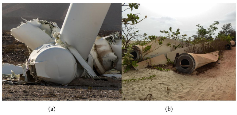
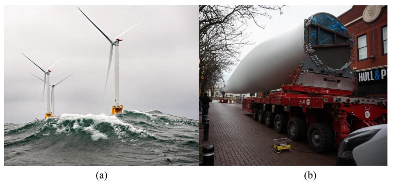
[6]	Siemens 2.37MW-108 SWT Wind Turbine Collapse in Ocotillo, 2016. Available from: https://www.flickr.com/photos/slworking/31210614186/in/photostream/.
[7]	Wind Turbine Blades Along a Road, Gambia, 2013. Available from: https://www.flickr.com/photos/jbdodane/.
[8]	Jaynes CH, Green Energy is Set to Match the World's Growing Electricity Demand-IEA Report. 2024. Available from: https://www.weforum.org/agenda/2024/02/green-energy-electricity-demand-growth-iea-report/.
[9]	Fernández L, Global Wind Power Market-Statistics & Facts. 2024. Available from: https://www.statista.com/topics/4564/global-wind-energy/#topicOverview.
[10]	WWEA Half-year Report 2023: Additional Momentum for Windpower in 2023. 2023. Available from: https://wwindea.org/wwea-half-year-report-2023-additional-momentum-for-windpower-in-2023.
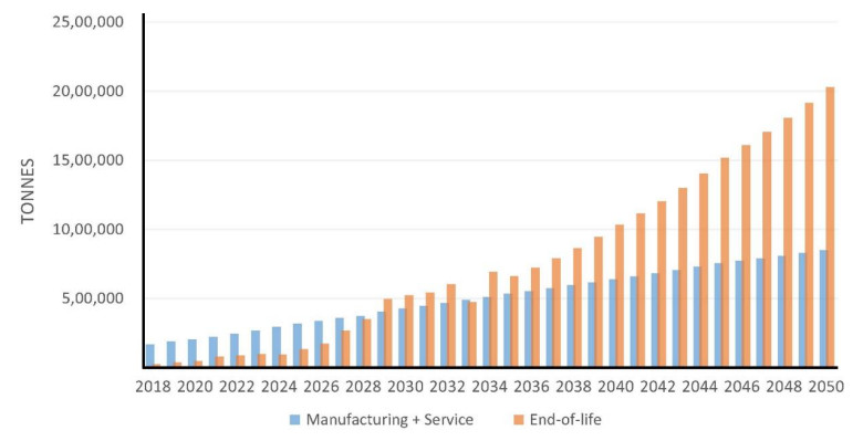
[11]	Heng H, Meng F, McKechnie J (2021) Wind turbine blade wastes and the environmental impacts in Canada. Waste Manag 133: 59–70. https://doi.org/10.1016/j.wasman.2021.07.032 doi: 10.1016/j.wasman.2021.07.032
[12]	Liu P, Barlow CY (2017) Wind turbine blade waste in 2050. Waste Manag 62: 229–240. https://doi.org/10.1016/j.wasman.2017.02.007 doi: 10.1016/j.wasman.2017.02.007
[13]	Canary Staff, 15 Companies Working to Recycle Wind Turbines, Solar Panels and Batteries. 2022. Available from: https://www.canarymedia.com/articles/clean-energy/15-companies-working-to-recycle-wind-turbines-solar-panels-and-batteries.
[14]	Americanrecycler Wind Turbine Blade Recycling Market to Reach $ \$ $5.6 Billion by 2033. Available from: https://americanrecycler.com/wind-turbine-blade-recycling-market-to-reach-usd-5-6-billion-by-2033/.
[15]	Shtayat A, Moridpour S, Best B, et al. (2020) A review of monitoring systems of pavement condition in paved and unpaved roads. J Traffic Transp Eng Engl Ed 7: 629–638. https://doi.org/10.1016/j.jtte.2020.03.004 doi: 10.1016/j.jtte.2020.03.004
[16]	Setyawan A, Irfansyah PA, Shidiq AM, et al. (2017) Design and properties of asphalt concrete mixtures using renewable bioasphalt binder. IOP Conf Ser Mater Sci Eng 176: 012028. https://doi.org/10.1088/1757-899X/176/1/012028 doi: 10.1088/1757-899X/176/1/012028
[17]	Ye Z (2021) Research on asphalt pavement diseases and construction quality control under the background of big data. J Phys Conf Ser 1744: 042139. https://doi.org/10.1088/1742-6596/1744/4/042139 doi: 10.1088/1742-6596/1744/4/042139
[18]	Taher SA, Alyousify S, Hassan HJA, et al. (2020) Comparative study of using flexible and rigid pavements for roads: A review study. J Univ Duhok 23: 222–234. https://doi.org/10.26682/csjuod.2020.23.2.18 doi: 10.26682/csjuod.2020.23.2.18
[19]	Yaro NSA, Sutanto MH, Baloo L, et al. (2023) A comprehensive overview of the utilization of recycled waste materials and technologies in asphalt pavements: Towards environmental and sustainable low-carbon roads. Processes 11: 2095. https://doi.org/10.3390/pr11072095 doi: 10.3390/pr11072095
[20]	Sulyman M, Sienkiewicz M, Haponiuk J (2014) Asphalt pavement material improvement: A review. Int J Environ Sci Dev 5: 444–454. https://doi.org/10.7763/IJESD.2014.V5.525 doi: 10.7763/IJESD.2014.V5.525
[21]	Rahman MT, Mohajerani A, Giustozzi F (2020) Recycling of waste materials for asphalt concrete and bitumen: A review. Materials 13: 1495. https://doi.org/10.3390/ma13071495 doi: 10.3390/ma13071495
[22]	Meijer JR, Huijbregts MAJ, Schotten KCGJ, et al. (2018) Global patterns of current and future road infrastructure. Environ Res Lett 13: 064006. https://doi.org/10.1088/1748-9326/aabd42 doi: 10.1088/1748-9326/aabd42
[23]	Price TJ (2006) UK large-scale wind power programme from 1970 to 1990: The carmarthen bay experiments and the musgrove vertical-axis turbines. Wind Eng 30: 225–242. https://doi.org/10.1260/030952406778606214 doi: 10.1260/030952406778606214
[24]	Gipe P, Möllerström E (2022) An overview of the history of wind turbine development: Part Ⅰ—The early wind turbines until the 1960s. Wind Eng 46: 1973–2004. https://journals.sagepub.com/doi/10.1177/0309524X221117825 doi: 10.1177/0309524X221117825
[25]	Kale SA, Kulkarni SR, Shravagi SD, et al. (2021) Materials for small wind turbine blades. Renew Energ Sustain Develop 43–54. https://doi.org/10.13140/RG.2.2.22099.09762 doi: 10.13140/RG.2.2.22099.09762
[26]	Bulent E, Aysegul A, Ali V (2006) Using of composite material in wind turbine blades. J Appl Sci 6: 2917–2921. https://doi.org/10.3923/jas.2006.2917.2921 doi: 10.3923/jas.2006.2917.2921
[27]	Olabi AG, Wilberforce T, Elsaid K, et al. (2021) A review on failure modes of wind turbine components. Energies 14: 5241. https://doi.org/10.3390/en14175241 doi: 10.3390/en14175241
[28]	Rajak D, Pagar D, Menezes P, et al. (2019) Fiber-reinforced polymer composites: Manufacturing, properties, and applications. Polymers 11: 1667. https://doi.org/10.3390/polym11101667 doi: 10.3390/polym11101667
[29]	Chan YWS, Zhou Z (2014) Advances of FRP-based smart components and structures. Pac Sci Rev 16: 1–7. https://doi.org/10.1016/j.pscr.2014.08.001 doi: 10.1016/j.pscr.2014.08.001
[30]	Jensen JP, Skelton K (2018) Wind turbine blade recycling: Experiences, challenges and possibilities in a circular economy. Renew Sustain Energy Rev 97: 165–176. https://doi.org/10.1016/j.rser.2018.08.041 doi: 10.1016/j.rser.2018.08.041
[31]	Mishnaevsky L, Branner K, Petersen H, et al. (2017) Materials for wind turbine blades: An overview. Materials 10: 1285. https://doi.org/10.3390/ma10111285 doi: 10.3390/ma10111285
[32]	Martin RW, Sabato A, Schoenberg A, et al. (2018) Comparison of nondestructive testing techniques for the inspection of wind turbine blades' spar caps. Wind Energy 21: 980–996. https://doi.org/10.1002/we.2208 doi: 10.1002/we.2208
[33]	Blain L, World's Largest Wind Turbine Is Now Fully Operational and Connected. 2023. Available from: https://newatlas.com/energy/worlds-largest-wind-turbine-myse-16-260/.
[34]	Cotrell J, Stehly T, Johnson J, et al. (2014) Analysis of transportation and logistics challenges affecting the deployment of larger wind turbines: Summary of results. Natl Renew Energ Lab 6664. https://doi.org/10.2172/1123207 doi: 10.2172/1123207
[35]	Dennis S, Heavy Seas Engulf the Block Island Wind Farm. 2016. Available from: https://www.flickr.com/photos/nrel/30353919862/in/photostream/.
[36]	Ian S, 75 Metre Wind Turbine Blade, 2017. Available from: https://commons.wikimedia.org/wiki/File: 75_metre_Wind_Turbine_Blade_-_geograph.org.uk_-_5247445.jpg.
[37]	Andersen PD, Bonou A, Beauson J, et al. (2014) Recycling of wind turbines, In: Larsen HH, Petersen LS, DTU International Energy Report 2014: Wind Energy—Drivers and Barriers for Higher Shares of Wind in the Global Power Generation Mix, Copenhagen: Technical University of Denmark. 91–97. https://orbit.dtu.dk/en/publications/recycling-ofwind-turbines
[38]	Sorte S, Martins N, Oliveira MSA, et al. (2023) Unlocking the potential of wind turbine blade recycling: Assessing techniques and metrics for sustainability. Energies 16: 7624. https://doi.org/10.3390/en16227624 doi: 10.3390/en16227624
[39]	Nanjegowda VH, Rathankumar MN, Anirudh N (2023) Fillers influence on hot-mix asphalt mixture design and performance assessment. IOP Conf Ser Earth Environ Sci 1149: 012013. https://doi.org/10.1088/1755-1315/1149/1/012013 doi: 10.1088/1755-1315/1149/1/012013
[40]	Fischer HR, Dillingh EC, Hermse CGM (2013) On the interfacial interaction between bituminous binders and mineral surfaces as present in asphalt mixtures. Appl Surf Sci 265: 495–499. https://doi.org/10.1016/j.apsusc.2012.11.034 doi: 10.1016/j.apsusc.2012.11.034
[41]	Mumtaz H, Sobek S, Sajdak M, et al. (2023) An experimental investigation and process optimization of the oxidative liquefaction process as the recycling method of the end-of-life wind turbine blades. Renew Energy 211: 269–278. https://doi.org/10.1016/j.renene.2023.04.120 doi: 10.1016/j.renene.2023.04.120
[42]	Lin J, Guo Z, Hong B, et al. (2022) Using recycled waste glass fiber reinforced polymer (GFRP) as filler to improve the performance of asphalt mastics. J Clean Prod 336: 130357. https://doi.org/10.1016/j.jclepro.2022.130357 doi: 10.1016/j.jclepro.2022.130357
[43]	Lan T, Wang B, Zhang J, et al. (2023) Utilization of waste wind turbine blades in performance improvement of asphalt mixture. Front Mater 10: 1164693. https://doi.org/10.3389/fmats.2023.1164693 doi: 10.3389/fmats.2023.1164693
[44]	Liao MC, Chen JS, Tsou KW (2012) Fatigue characteristics of bitumen-filler mastics and asphalt mixtures. J Mater Civ Eng 24: 916–923. https://doi.org/10.1061/(ASCE)MT.1943-5533.0000450 doi: 10.1061/(ASCE)MT.1943-5533.0000450
[45]	Zhen T, Zhao P, Zhang X, et al. (2023) The effect of GFRP powder on the high and low-temperature properties of asphalt mastic. Materials 16: 2662. https://doi.org/10.3390/ma16072662 doi: 10.3390/ma16072662
[46]	Liu G, Yang T, Li J, et al. (2018) Effects of aging on rheological properties of asphalt materials and asphalt-filler interaction ability. Constr Build Mater 168: 501–511. https://doi.org/10.1016/j.conbuildmat.2018.02.171 doi: 10.1016/j.conbuildmat.2018.02.171
[47]	Yang W, Kim KH, Lee J (2022) Upcycling of decommissioned wind turbine blades through pyrolysis. J Clean Prod 376: 134292. https://doi.org/10.1016/j.jclepro.2022.134292 doi: 10.1016/j.jclepro.2022.134292
[48]	Xu M, Ji H, Wu Y, et al. (2023) The pyrolysis of end-of-life wind turbine blades under different atmospheres and their effects on the recovered glass fibers. Compos Part B Eng 251: 110493. https://doi.org/10.1016/j.compositesb.2022.110493 doi: 10.1016/j.compositesb.2022.110493
[49]	Åkesson D, Foltynowicz Z, Christéen J, et al. (2012) Microwave pyrolysis as a method of recycling glass fibre from used blades of wind turbines. J Reinf Plast Compos 31: 1136–1142. https://doi.org/10.1177/0731684412453512 doi: 10.1177/0731684412453512
[50]	Mishnaevsky L (2021) Sustainable end-of-life management of wind turbine blades: Overview of current and coming solutions. Materials 14: 1124. https://doi.org/10.3390/ma14051124 doi: 10.3390/ma14051124
[51]	Protsenko AE, Protsenko AN, Shakirova OG, et al. (2023) Recycling of epoxy/fiberglass composite using supercritical ethanol with (2, 3, 5-Triphenyltetrazolium)₂[CuCl₄] complex. Polymers 15: 1559. https://doi.org/10.3390/polym15061559 doi: 10.3390/polym15061559
[52]	Mattsson C, André A, Juntikka M, et al. (2020) Chemical recycling of end-of-life wind turbine blades by solvolysis/HTL. IOP Conf Ser Mater Sci Eng 942: 012013. https://doi.org/10.1088/1757-899X/942/1/012013 doi: 10.1088/1757-899X/942/1/012013
[53]	Sokoli HU (2016) Chemical solvolysis as an approach to recycle fibre reinforced thermoset polymer composites and close the end-of the life cycle. Aalborg University https://doi.org/10.5278/VBN.PHD.ENGSCI.00171 doi: 10.5278/VBN.PHD.ENGSCI.00171
[54]	Pickering SJ, Kelly RM, Kennerley JR, et al. (2000) A fluidised-bed process for the recovery of glass fibres from scrap thermoset composites. Compos Sci Technol 60: 509–523. https://doi.org/10.1016/S0266-3538(99)00154-2 doi: 10.1016/S0266-3538(99)00154-2
[55]	Oliveux G, Bailleul JL, Salle ELG (2012) Chemical recycling of glass fibre reinforced composites using subcritical water. Compos Part Appl Sci Manuf 43: 1809–1818. https://doi.org/10.1016/j.compositesa.2012.06.008 doi: 10.1016/j.compositesa.2012.06.008
[56]	Yang Q, Fan Z, Yang X, et al. (2023) Recycling waste fiber-reinforced polymer composites for low-carbon asphalt concrete: The effects of recycled glass fibers on the durability of bituminous composites. J Clean Prod 423: 138692. https://doi.org/10.1016/j.jclepro.2023.138692 doi: 10.1016/j.jclepro.2023.138692
[57]	Khater A, Luo D, Abdelsalam M, et al. (2021) Laboratory evaluation of asphalt mixture performance using composite admixtures of lignin and glass fibers. Appl Sci 11: 364. https://doi.org/10.3390/app11010364 doi: 10.3390/app11010364
[58]	Mahrez A, Karim MR, Katman HY (2005) Fatigue and deformation properties of glass fiber reinforced bituminous mixes. J Eastern Asia Society Transport Studies 6: 997–1007. https://doi.org/10.11175/easts.6.997 doi: 10.11175/easts.6.997
[59]	Jiao Y, Du W, Yang H, et al. (2024) Low temperature failure behavior analysis of fiber reinforced asphalt concrete under indirect tension test using acoustic emission and digital image correlation. Case Stud Constr Mater 20: e02720. https://doi.org/10.1016/j.cscm.2023.e02720 doi: 10.1016/j.cscm.2023.e02720
[60]	Ortega-López V, Faleschini F, Hurtado-Alonso N, et al. (2024) Analysis of raw-crushed wind-turbine blade as an overall concrete addition: Stress–strain and deflection performance effects. Compos Struct 340: 118170. https://doi.org/10.1016/j.compstruct.2024.118170 doi: 10.1016/j.compstruct.2024.118170
[61]	Yazdanbakhsh A, Bank LC, Rieder KA, et al. (2018) Concrete with discrete slender elements from mechanically recycled wind turbine blades. Resour Conserv Recycl 128: 11–21. https://doi.org/10.1016/j.resconrec.2017.08.005 doi: 10.1016/j.resconrec.2017.08.005
[62]	Baturkin D, Hisseine OA, Masmoudi R, et al. (2022) Compressive behavior of FRP-tube-confined concrete short columns using recycled FRP materials from wind turbine blades: Experimental investigation and analytical modelling. Clean Technol Recycl 2: 136–164. https://doi.org/10.3934/ctr.2022008 doi: 10.3934/ctr.2022008
[63]	Fu B, Liu KC, Chen JF, et al. (2021) Concrete reinforced with macro fibres recycled from waste GFRP. Constr Build Mater 310: 125063. https://doi.org/10.1016/j.conbuildmat.2021.125063 doi: 10.1016/j.conbuildmat.2021.125063
[64]	Baturkin D, Hisseine OA, Masmoudi R, et al. (2021) Valorization of recycled FRP materials from wind turbine blades in concrete. Resour Conserv Recycl 174: 105807. https://doi.org/10.1016/j.resconrec.2021.105807 doi: 10.1016/j.resconrec.2021.105807
[65]	Akbar A, Liew KM (2020) Assessing recycling potential of carbon fiber reinforced plastic waste in production of eco-efficient cement-based materials. J Clean Prod 274: 123001. https://doi.org/10.1016/j.jclepro.2020.123001 doi: 10.1016/j.jclepro.2020.123001
[66]	Ruane K, Zhang Z, Nagle A, et al. (2022) Material and structural characterization of a wind turbine blade for use as a bridge girder. Transport Res Rec 2676: 354–362. https://doi.org/10.1177/03611981221083619 doi: 10.1177/03611981221083619
[67]	Ruane K, Soutsos M, Huynh A, et al. (2023) Construction and cost analysis of bladebridges made from decommissioned FRP wind turbine blades. Sustainability 15: 3366. https://doi.org/10.3390/su15043366 doi: 10.3390/su15043366
[68]	Broniewicz M, Broniewicz F, Dec K, et al. (2024) The concept of using wind turbine propellers in the construction of acoustic screens as an example of a circular economy model. Econ Environ 87: 1–18. https://doi.org/10.34659/eis.2023.87.4.726 doi: 10.34659/eis.2023.87.4.726
[69]	Revilla-Cuesta V, Skaf M, Ortega-López V, et al. (2023) Raw-crushed wind-turbine blade: Waste characterization and suitability for use in concrete production. Resour Conserv Recycl 198: 107160. https://doi.org/10.1016/j.resconrec.2023.107160 doi: 10.1016/j.resconrec.2023.107160
[70]	André A, Kullberg J, Nygren D, et al. (2020) Re-use of wind turbine blade for construction and infrastructure applications. IOP Conf Ser Mater Sci Eng 942: 012015. https://doi.org/10.1088/1757-899X/942/1/012015 doi: 10.1088/1757-899X/942/1/012015
[71]	Martini R, Xydis G (2023) Repurposing and recycling wind turbine blades in the United States. Environ Prog Sustain 42: e13932. https://doi.org/10.1002/ep.13932 doi: 10.1002/ep.13932
[72]	Bank L, Arias F, Yazdanbakhsh A, et al. (2018) Concepts for reusing composite materials from decommissioned wind turbine blades in affordable housing. Recycling 3: 3. https://doi.org/10.3390/recycling3010003 doi: 10.3390/recycling3010003
[73]	McGlasson R, These Awesome Playgrounds Are Made Out of Old, Used-Up Wind Turbines—Here's Why That's Special. 2023. Available from: https://www.thecooldown.com/green-tech/blade-made-playground-wind-turbine-blades-recycled/.
[74]	Yelland C, Denmark Is Repurposing Discarded Wind Turbine Blades As Bike Shelters. 2021. Available from: https://www.designboom.com/design/denmark-repurposing-wind-turbine-blades-bike-garages-09-27-2021/.
[75]	Cherrington R, Goodship V, Meredith J, et al. (2012) Producer responsibility: Defining the incentive for recycling composite wind turbine blades in Europe. Energy Policy 47: 13–21. https://doi.org/10.1016/j.enpol.2012.03.076 doi: 10.1016/j.enpol.2012.03.076
[76]	Spini F, Bettini P (2024) End-of-Life wind turbine blades: Review on recycling strategies. Compos Part B Eng 275: 111290. https://doi.org/10.1016/j.compositesb.2024.111290 doi: 10.1016/j.compositesb.2024.111290
[77]	Cooperman A, Eberle A, Lantz E (2021) Wind turbine blade material in the United States: Quantities, costs, and end-of-life options. Resour Conserv Recycl 168: 105439. https://doi.org/10.1016/j.resconrec.2021.105439 doi: 10.1016/j.resconrec.2021.105439
[78]	Hasheminezhad A, Nazari Z, Yang B, et al. (2024) A comprehensive review of sustainable solutions for reusing wind turbine blade waste materials. J Environ Manage 366: 121735. https://doi.org/10.1016/j.jenvman.2024.121735 doi: 10.1016/j.jenvman.2024.121735
[79]	Tyurkay A, Kirkelund GM, Lima ATM (2024) State-of-the-art circular economy practices for end-of-life wind turbine blades for use in the construction industry. Sustain Prod Consum 47: 17–36. https://doi.org/10.1016/j.spc.2024.03.018 doi: 10.1016/j.spc.2024.03.018

Reader Comments

Your name:*

Email:*
© 2024 the Author(s), licensee AIMS Press. This is an open access article distributed under the terms of the Creative Commons Attribution License (http://creativecommons.org/licenses/by/4.0)