This research presents a novel optimization modeling framework for the existing Soil and Water Assessment Tool (SWAT), which can be used to optimize perennial feedstock production. This novel multi-objective evolutionary algorithm (MOEA) uses SWAT outputs to determine optimal spatial placement of variant cropping systems, considering environmental impacts from land-cover change and management practices. The final solution to the multi-objective problem is presented as a set of Pareto optimal solutions, where one is suggested considering the proximity to the ideal vector [1,0,0,0]. This unique approach provides a well-suited method to assist researchers and stakeholders in understanding the environmental impacts when cultivating biofuel feedstocks. The application of the proposed MOEA is illustrated by analyzing SWAT's example data set for Lake Fork Watershed. Nine land-cover scenarios were evaluated in SWAT to determine their optimal spatial placement considering maximizing biomass production while minimizing sediment yield, organic nitrogen yield, and organic phosphorous yield.
Citation: Ana Cram, Jose Espiritu, Heidi Taboada, Delia J. Valles-Rosales, Young Ho Park, Efren Delgado, Jianzhong Su. Multi-objective biofuel feedstock optimization considering different land-cover scenarios and watershed impacts[J]. Clean Technologies and Recycling, 2022, 2(2): 103-118. doi: 10.3934/ctr.2022006
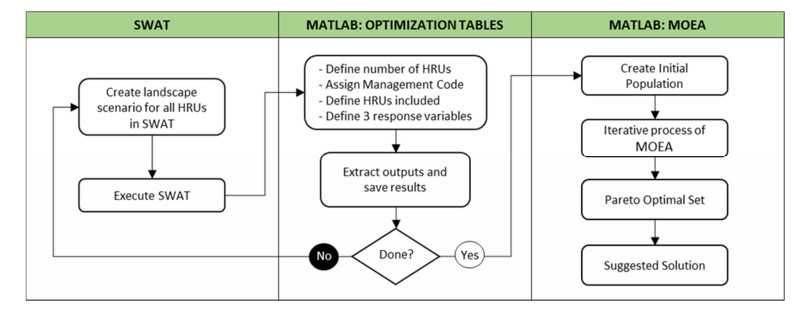
This research presents a novel optimization modeling framework for the existing Soil and Water Assessment Tool (SWAT), which can be used to optimize perennial feedstock production. This novel multi-objective evolutionary algorithm (MOEA) uses SWAT outputs to determine optimal spatial placement of variant cropping systems, considering environmental impacts from land-cover change and management practices. The final solution to the multi-objective problem is presented as a set of Pareto optimal solutions, where one is suggested considering the proximity to the ideal vector [1,0,0,0]. This unique approach provides a well-suited method to assist researchers and stakeholders in understanding the environmental impacts when cultivating biofuel feedstocks. The application of the proposed MOEA is illustrated by analyzing SWAT's example data set for Lake Fork Watershed. Nine land-cover scenarios were evaluated in SWAT to determine their optimal spatial placement considering maximizing biomass production while minimizing sediment yield, organic nitrogen yield, and organic phosphorous yield.

| [1] | Congress US, Energy Independence and Security Act of 2007. Public Law 110-140. Congress Washington DC, 2007. Available from: https://uscode.house.gov/statutes/pl/110/140.pdf. |
| [2] | Neitsch SL, Arnold JG, Kiniry JR, et al. (2011) Soil and Water Assessment Tool theoretical documentation version 2009. Texas Water Resources Institute Technical Report no. 406. Available from: https://oaktrust.library.tamu.edu/handle/1969.1/128050. |
| [3] | Economic Research Service (ERS), U.S. Department of Agriculture (USDA). Food Environment Atlas, 2022. Available from: https://www.ers.usda.gov/data-products/us-bioenergy-statistics/. |
| [4] | National Research Council (2008) Water Implications of Biofuels Production in the United States, Washington DC: National Academies Press. |
| [5] | Eghball B, Gilley JE, Kramer LA, et al. (2000) Narrow grass hedge effects on phosphorus and nitrogen in runoff following manure and fertilizer application. J Soil Water Conserv 55: 172-176. |
| [6] | Turner RE, Rabalais NN, Dortch Q, et al. (1995) Evidence for nutrient limitation on sources causing hypoxia on the Louisiana shelf, Proceedings of the 1st Gulf of Mexico Hypoxia Management Conference, 106-112. |
| [7] |
Blanco‐Canqui H (2010) Energy crops and their implications on soil and environment. Agron J 102: 403-419. https://doi.org/10.2134/agronj2009.0333 doi: 10.2134/agronj2009.0333

|
| [8] |
McGregor KC, Dabney S, Johnson JR (1999) Runoff and soil loss from cotton plotswith and without stiff-grass hedges. Trans ASAE 42: 361-368. https://doi.org/10.13031/2013.13367 doi: 10.13031/2013.13367
|
| [9] |
Blanco-Canqui H, Gantzer CJ, Anderson SH, et al. (2004) Grass barriers for reduced concentrated flow induced soil and nutrient loss. Soil Sci Soc Am J 68: 1963-1972. https://doi.org/10.2136/sssaj2004.1963 doi: 10.2136/sssaj2004.1963
|
| [10] |
Blanco-Canqui H, Gantzer CJ, Anderson SH, et al. (2004) Grass barrier and vegetative filter strip effectiveness in reducing runoff, sediment, nitrogen, and phosphorus loss. Soil Sci Soc Am J 68: 1670-1678. https://doi.org/10.2136/sssaj2004.1670 doi: 10.2136/sssaj2004.1670
|
| [11] |
Blanco‐Canqui H (2010) Energy crops and their implications on soil and environment. Agron J 102: 403-419. https://doi.org/10.2134/agronj2009.0333 doi: 10.2134/agronj2009.0333
|
| [12] | Hannah L, Lovejoy TE, Schneider SH (2019) Biodiversity and climate change in context, Climate Change and Biodiversity, New Haven: Yale University Press. https://doi.org/10.2307/j.ctv8jnzw1 |
| [13] |
Tallis H, Polasky S (2009) Mapping and valuing ecosystem services as an approach for conservation and natural‐resource management. Ann NY Acad Sci 1162: 265-283. https://doi.org/10.1111/j.1749-6632.2009.04152.x doi: 10.1111/j.1749-6632.2009.04152.x
|
| [14] |
Engel B, Chaubey I, Thomas M, et al. (2010) Biofuels and water quality: challenges and opportunities for simulation modeling. Biofuels 1: 463-477. https://doi.org/10.4155/bfs.10.17 doi: 10.4155/bfs.10.17
|
| [15] |
Gallardo-Vázquez D, Valdez-Juárez LE, Lizcano-Á lvarez JL (2019) Corporate social responsibility and intellectual capital: Sources of competitiveness and legitimacy in organizations' management practices. Sustainability 11: 5843. https://doi.org/10.3390/su11205843 doi: 10.3390/su11205843
|
| [16] |
Nä schen K, Diekkrüger B, Evers M, et al. (2019) The impact of land use/land cover change (LULCC) on water resources in a tropical catchment in Tanzania under different climate change scenarios. Sustainability 11: 7083. https://doi.org/10.3390/su11247083 doi: 10.3390/su11247083
|
| [17] |
Tang C, Li J, Zhou Z, et al. (2019) How to optimize ecosystem services based on a Bayesian model: A case study of Jinghe River Basin. Sustainability 11: 4149. https://doi.org/10.3390/su11154149 doi: 10.3390/su11154149
|
| [18] | Kaini P, Artita K, Nicklow JW (2007) Evaluating optimal detention pond locations at a watershed scale, World Environmental and Water Resources Congress 2007: Restoring Our Natural Habitat, 1-8. https://doi.org/10.1061/40927(243)170 |
| [19] |
Kaini P, Artita K, Nicklow JW (2012) Optimizing structural best management practices using SWAT and genetic algorithm to improve water quality goals. Water Resour Manag 26: 1827-1845. https://doi.org/10.1007/s11269-012-9989-0 doi: 10.1007/s11269-012-9989-0
|
| [20] | Kaini P, Artita K, Nicklow JW (2009) Generating different scenarios of BMP designs in a watershed scale by combining NSGA-II with SWAT, World Environmental and Water Resources Congress 2009: Great Rivers, 1-9. https://doi.org/10.1061/41036(342)493 |
| [21] | Artita KS, Kaini P, Nicklow JW (2008) Generating alternative watershed-scale BMP designs with evolutionary algorithms, World Environmental and Water Resources Congress 2008: Ahupua'A, 1-9. https://doi.org/10.1061/40976(316)127 |
| [22] |
Maringanti C, Chaubey I, Arabi M, et al. (2008) A multi-objective optimization tool for the selection and placement of BMPs for pesticide control. Hydrol Earth Syst Sci Discuss 5: 28-29. https://doi.org/10.5194/hessd-5-1821-2008 doi: 10.5194/hessd-5-1821-2008
|
| [23] |
Maringanti C, Chaubey I, Arabi M, et al. (2011) Application of a multi-objective optimization method to provide least cost alternatives for NPS pollution control. Environ Manage 48: 448-461. https://doi.org/10.1007/s00267-011-9696-2 doi: 10.1007/s00267-011-9696-2
|
| [24] |
Herman MR, Nejadhashemi AP, Daneshvar F, et al. (2016) Optimization of bioenergy crop selection and placement based on a stream health indicator using an evolutionary algorithm. J Environ Manage 181: 413-424. https://doi.org/10.1016/j.jenvman.2016.07.005 doi: 10.1016/j.jenvman.2016.07.005
|
| [25] |
Gitau MW, Veith TL, Gburek WJ (2004) Farm-level optimization of BMP placement for cost-effective pollution reduction. Trans ASAE 47: 1923-1931. https://doi.org/10.13031/2013.17805 doi: 10.13031/2013.17805
|
| [26] |
Gitau MW, Veith TL, Gburek WJ, et al. (2006) Watershed level best management practice selection and placement in the Town Brook Watershed, New York. J Am Water Resour As 42: 1565-1581. https://doi.org/10.1111/j.1752-1688.2006.tb06021.x doi: 10.1111/j.1752-1688.2006.tb06021.x
|
| [27] |
Muleta MK, Nicklow JW (2002) Evolutionary algorithms for multiobjective evaluation of watershed management decisions. J Hydroinf 4: 83-97. https://doi.org/10.2166/hydro.2002.0010 doi: 10.2166/hydro.2002.0010
|
| [28] |
Ng TL, Eheart JW, Cai X, et al. (2010) Modeling Miscanthus in the Soil and Water Assessment Tool (SWAT) to simulate its water quality effects as a bioenergy crop. Environ Sci Technol 44: 7138-7144. https://doi.org/10.1021/es9039677 doi: 10.1021/es9039677
|
| [29] | USDA Plants Database, Natural Resources Conservation Service. United States Department of Agriculture, 2022. Available from: https://plants.usda.gov/home. |
| [30] |
Taboada HA, Coit DW (2012) A new multiple objective evolutionary algorithm for reliability optimization of series-parallel systems. Int J Appl Evol Comput 3: 1-18. https://doi.org/10.4018/jaec.2012040101 doi: 10.4018/jaec.2012040101
|
| [31] |
Gassman PW, Reyes MR, Green CH, et al. (2007) The Soil and Water Assessment Tool: historical development, applications, and future research directions. Trans ASABE 50: 1211-1250. https://doi.org/10.13031/2013.23637 doi: 10.13031/2013.23637
|
| [32] | Arnold JG, Kiniry JR, Srinivasan R, et al. (2013) SWAT 2012 Input/Output Documentation. Texas Water Resources Institute. Available from: https://oaktrust.library.tamu.edu/handle/1969.1/149194. |
| [33] | Winchell M, Srinivasan R, Di Luzio M, et al. (2010) ArcSWAT interface for SWAT 2009, User's Guide, Blackland Research Center, Texas Agricultural Experiment Station, Temple. |


Figures(8) / Tables(2)
Ana Cram, Jose Espiritu, Heidi Taboada, Delia J. Valles-Rosales, Young Ho Park, Efren Delgado, Jianzhong Su. Multi-objective biofuel feedstock optimization considering different land-cover scenarios and watershed impacts[J]. Clean Technologies and Recycling, 2022, 2(2): 103-118. doi: 10.3934/ctr.2022006


 DownLoad: