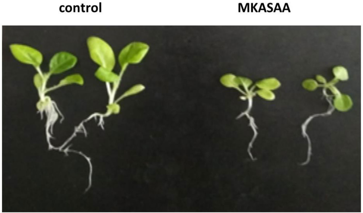
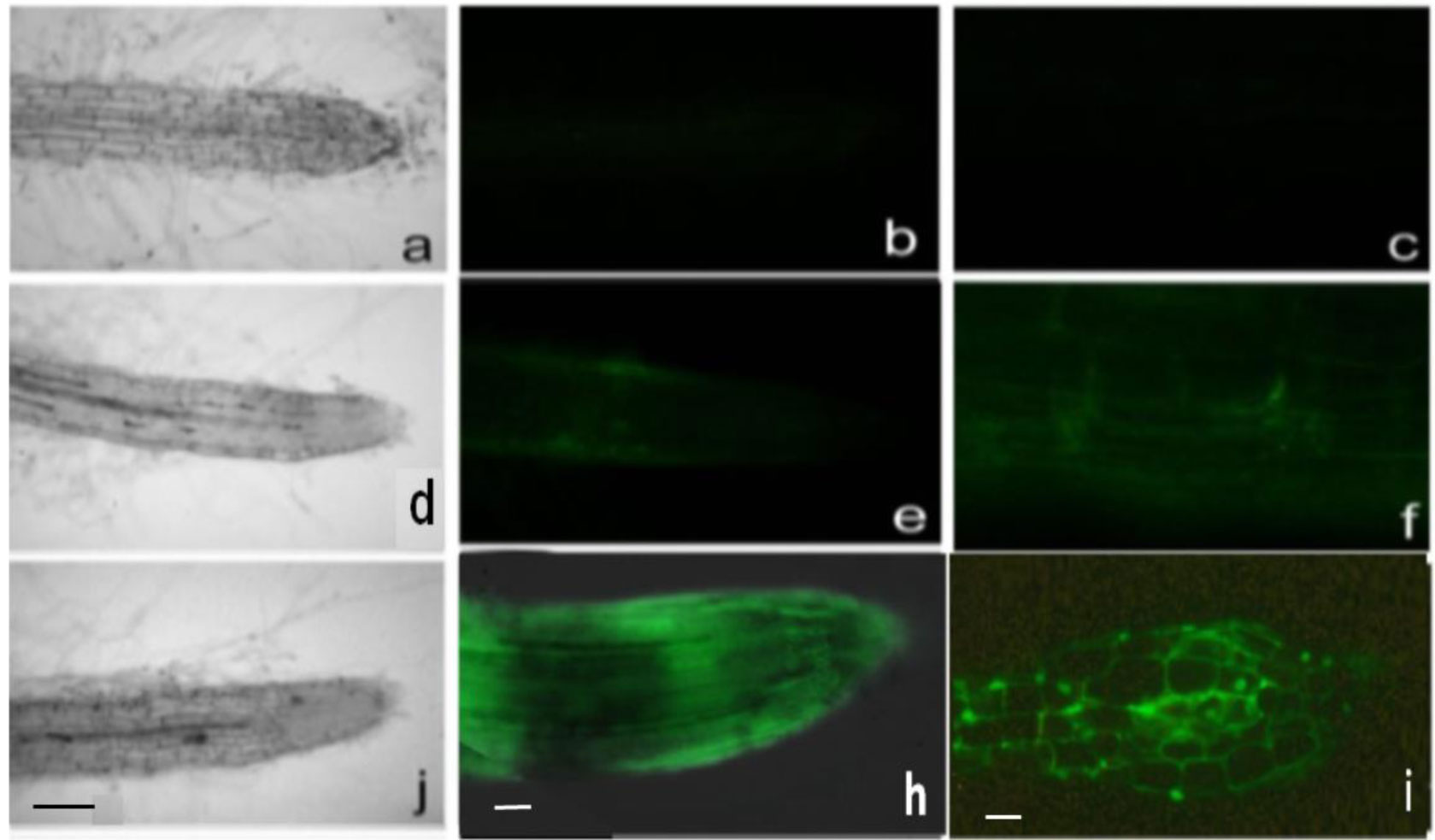
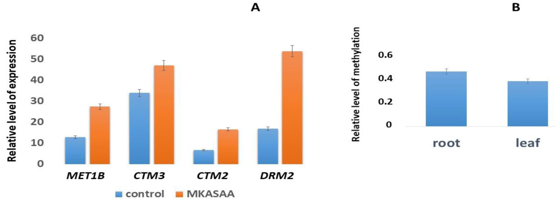
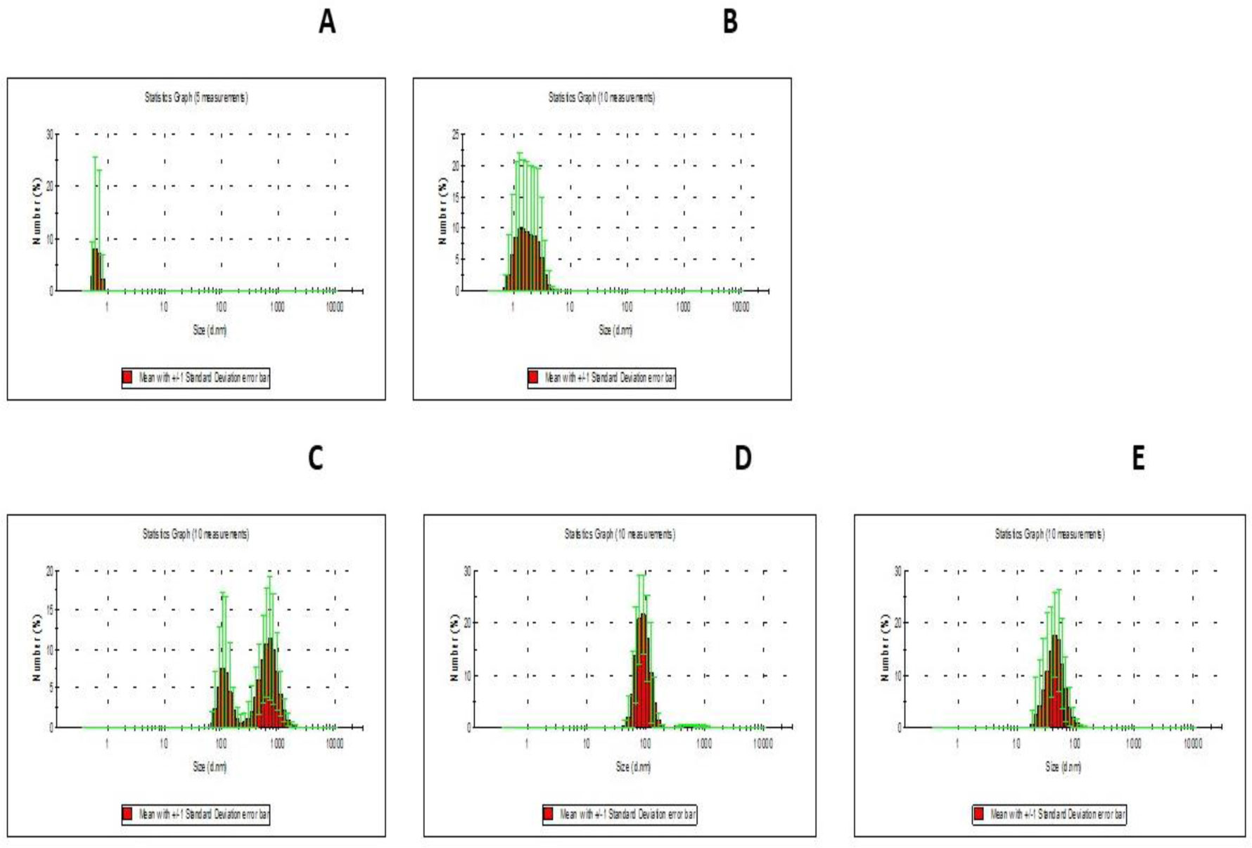
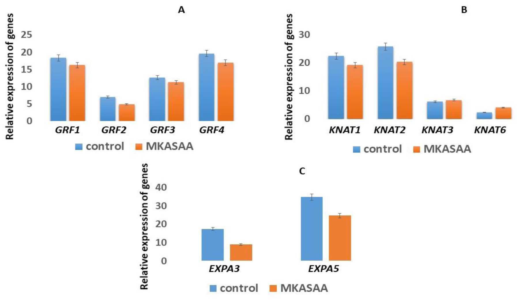
DNA methylation is involved in the protection of the genome, the regulation of gene expression, splicing, and is associated with a serious reprogramming of plant development. Using fluorescence microscopy, it was shown that the MKASAA peptide penetrates through the root system of Nicotiana tabacum tobacco, mainly into the cap, meristem, and elongation zones. In the cell, the peptide is localized mainly on the nuclei. In tobacco seedlings grown in the presence of the peptide at a concentration of 10–7 M, an increase in the expression of DNA methyltransferases, especially DRM2, which methylates previously unmethylated DNA sites, is observed. In the presence of the peptide in the roots and leaves of tobacco, the level of global DNA methylation increases. An increase in DNA methylation occurs via the RdDM pathway. Presumably, the peptide binds to siRNAs, forming giant particles that remodulate chromatin and facilitate the entry of DNA methyltransferases. An increase in the level of DNA methylation is accompanied by silencing of the genes of the GRF, KNOX, and EXP families. Suppression of gene expression of these families is accompanied by significant morphological changes in tobacco seedlings. Thus, the short exogenous MKASAA peptide is involved in global morphological and genetic changes in tobacco seedlings.
Citation: Larisa I. Fedoreyeva, Tatiana A. Dilovarova, Boris F. Vanyushin, Inna A. Chaban, Neonila V. Kononenko. Regulation of gene expression in Nicotiana tabacum seedlings by the MKASAA peptide through DNA methylation via the RdDM pathway[J]. AIMS Biophysics, 2022, 9(2): 113-129. doi: 10.3934/biophy.2022011
DNA methylation is involved in the protection of the genome, the regulation of gene expression, splicing, and is associated with a serious reprogramming of plant development. Using fluorescence microscopy, it was shown that the MKASAA peptide penetrates through the root system of Nicotiana tabacum tobacco, mainly into the cap, meristem, and elongation zones. In the cell, the peptide is localized mainly on the nuclei. In tobacco seedlings grown in the presence of the peptide at a concentration of 10–7 M, an increase in the expression of DNA methyltransferases, especially DRM2, which methylates previously unmethylated DNA sites, is observed. In the presence of the peptide in the roots and leaves of tobacco, the level of global DNA methylation increases. An increase in DNA methylation occurs via the RdDM pathway. Presumably, the peptide binds to siRNAs, forming giant particles that remodulate chromatin and facilitate the entry of DNA methyltransferases. An increase in the level of DNA methylation is accompanied by silencing of the genes of the GRF, KNOX, and EXP families. Suppression of gene expression of these families is accompanied by significant morphological changes in tobacco seedlings. Thus, the short exogenous MKASAA peptide is involved in global morphological and genetic changes in tobacco seedlings.

| [1] |
Eichten SR, Schmitz RJ, Springer NM (2014) Epigenetics: beyond chromatin modifications and complex genetic regulation. Plant Physiol 165: 933-947. https://doi.org/10.1104/pp.113.234211 
|
| [2] |
Bannister AJ, Kouzarides T (2011) Regulation of chromatin by histone modifications. Cell Res 21: 381-395. https://doi.org/10.1038/cr.2011.22
|
| [3] |
Jerzmanowski A (2007) SWI/SNF chromatin remodeling and linker histones in plants. BBA-Gene Struct and Expres 1769: 330-345. https://doi.org/10.1016/j.bbaexp.2006.12.003
|
| [4] |
Jaenisch R, Bird A (2003) Epigenetic regulation of gene expression: how the genome integrates intrinsic and environmental signals. Nat Genet 33: 245-254. https://doi.org/10.1038/ng1089
|
| [5] |
Minard ME, Jain AK, Barton MC (2009) Analysis of epigenetic alterations to chromatin during development. Genesis 47: 559-572. https://doi.org/10.1002/dvg.20534
|
| [6] |
Jenuwein T, Allis CD (2001) Translating the histone code. Science 293: 1074-1080. https://doi.org/10.1126/science.1063127
|
| [7] |
Fischle W, Wang Y, Allis CD (2003) Histone and chromatin cross-talk. Curr Opin Cell Biol 15: 172-183. https://doi.org/10.1016/S0955-0674(03)00013-9
|
| [8] |
Goll MG, Bestor TH (2005) Eukaryotic cytosine methyltransferases. Annu Rev Biochem 74: 481.
|
| [9] |
Lister R, Pelizzola M, Dowen RH, et al. (2009) Human DNA methylomes at base resolution show widespread epigenomic differences. Nature 462: 315-322. https://doi.org/10.1038/nature08514
|
| [10] |
Lister R, Mukamel EA, Nery JR, et al. (2013) Global epigenomic reconfiguration during mammalian brain development. Science 341: 1237905. https://doi.org/10.1126/science.1237905
|
| [11] |
Erdmann RM, Picard CL (2020) RNA-directed DNA methylation. PLoS Genet 16: e1009034. https://doi.org/10.1371/journal.pgen.1009034
|
| [12] |
Du J, Johnson LM, Jacobsen SE, et al. (2015) DNA methylation pathways and their crosstalk with histone methylation. Nat Rev Mol Cell Biol 16: 519-532. https://doi.org/10.1038/nrm4043
|
| [13] |
Klemm SL, Shipony Z, Greenleaf WJ (2019) Chromatin accessibility and the regulatory epigenome. Nat Rev Genet 20: 207-220. https://doi.org/10.1038/s41576-018-0089-8
|
| [14] | Fortes AM, Gallusci P (2017) Plant stress responses and phenotypic plasticity in the epigenomics era: perspectives on the grapevine scenario, a model for perennial crop plants. Front Plant Sci 8: 82. https://doi.org/10.3389/fpls.2017.00082 |
| [15] |
Kumar A, Bennetzen JL (1999) Plant retrotransposons. Annu Rev Genet 33: 479-532.
|
| [16] |
Ito H, Kim JM, Matsunaga W, et al. (2016) A stress-activated transposon in Arabidopsis induces transgenerational abscisic acid insensitivity. Sci Rep 6: 23181. https://doi.org/10.1038/srep23181
|
| [17] |
Hsiao YC, Yamada M (2021) The roles of peptide hormones and their receptors during plant root development. Genes 12: 22. https://doi.org/10.3390/genes12010022
|
| [18] |
Fedoreyeva LI, Dilovarova TA, Kononenko NV, et al. (2018) Influence of glycylglycine, glycine, and glycylaspartic acid on growth, development, and gene expression in a tobacco (Nicotiana tabacum) callus culture. Biol Bull 45: 351-358. https://doi.org/10.1134/S1062359018040039
|
| [19] |
Kononenko N, Baranova E, Dilovarova T, et al. (2020) Oxidative damage to various root and shoot tissues of durum and soft wheat seedlings during salinity. Agriculture 10: 55. https://doi.org/10.3390/agriculture10030055
|
| [20] |
Bell K, Mitchell S, Paultre D, et al. (2013) Correlative imaging of fluorescent proteins in resin-embedded plant material. Plant Physiol 161: 1595-1603. https://doi.org/10.1104/pp.112.212365
|
| [21] |
Fedoreyeva LI, Vanyushin BF, Baranova EN (2020) Peptide AEDL alters chromatin conformation via histone binding. AIMS Biophys 7: 1-16.
|
| [22] |
Favicchio R, Dragan AI, Kneale GG, et al. (2009) Fluorescence spectroscopy and anisotropy in the analysis of DNA-protein interactions. DNA-Protein Interactions 543: 589-611. https://doi.org/10.1007/978-1-60327-015-1_35
|
| [23] |
Hsiao YC, Yamada M (2021) The roles of peptide hormones and their receptors during plant root development. Genes 12: 22. https://doi.org/10.3390/genes12010022
|
| [24] |
Gantt JS, Lenvik TR (1991) Arabidopsis thaliana H1 histones: analysis of two members of a small gene family. Eur J Biochem 202: 1029-1039. https://doi.org/10.1111/j.1432-1033.1991.tb16466.x
|
| [25] |
McGinty RK, Tan S (2015) Nucleosome structure and function. Chem Rev 115: 2255-2273. https://doi.org/10.1021/cr500373h
|
| [26] |
Cuerda-Gil D, Slotkin RK (2016) Non-canonical RNA-directed DNA methylation. Nat Plants 2: 16163. https://doi.org/10.1038/nplants.2016.163
|
| [27] |
Matzke MA, Kanno T, Matzke AJM (2015) RNA-directed DNA methylation: the evolution of a complex epigenetic pathway in flowering plants. Annu Rev Plant Biol 66: 243-267. https://doi.org/10.1146/annurev-arplant-043014-114633
|
| [28] | Wendte JM, Pikaard CS (2017) The RNAs of RNA-directed DNA methylation. BBA-Gene Regul Mech 1860: 140-148. https://doi.org/10.1016/j.bbagrm.2016.08.004 |
| [29] |
Matzke MA, Mosher RA (2014) RNA-directed DNA methylation: an epigenetic pathway of increasing complexity. Nat Rev Genet 15: 394-408. https://doi.org/10.1038/nrg3683
|
| [30] |
Cao X, Jacobsen SE (2002) Role of the Arabidopsis DRM methyltransferases in de novo DNA methylation and gene silencing. Curr Biol 12: 1138-1144. https://doi.org/10.1016/S0960-9822(02)00925-9
|
| [31] |
Omidbakhshfard MA, Proost S, Fujikura U, et al. (2015) Growth-regulating factors (GRFs): a small transcription factor family with important functions in plant biology. Mol Plant 8: 998-1010. https://doi.org/10.1016/j.molp.2015.01.013
|
| [32] |
Kuijt SJH, Greco R, Agalou A, et al. (2014) Interaction between the GROWTH-REGULATING FACTOR and KNOTTED1-LIKE HOMEOBOX families of transcription factors. Plant Physiol 164: 1952-1966. https://doi.org/10.1104/pp.113.222836
|
| [33] |
Srinivasan C, Liu Z, Scorza R (2011) Ectopic expression of class 1 KNOX genes induce adventitious shoot regeneration and alter growth and development of tobacco (Nicotiana tabacum L) and European plum (Prunus domestica L). Plant Cell Rep 30: 655-664. https://doi.org/10.1007/s00299-010-0993-7
|
| [34] |
Zhang W, Yu R (2014) Molecule mechanism of stem cells in Arabidopsis thaliana. Pharmacogn Rev 8: 105-112. https://doi.org/10.4103%2F0973-7847.134243
|
| [35] |
Long JA, Moan EI, Medford JI, et al. (1996) A member of the KNOTTED class of homeodomain proteins encoded by the STM gene of Arabidopsis. Nature 379: 66-69. https://doi.org/10.1038/379066a0
|
| [36] |
Belles-Boix E, Hamant O, Witiak SM, et al. (2006) KNAT6: an Arabidopsis homeobox gene involved in meristem activity and organ separation. Plant Cell 18: 1900-1907. https://doi.org/10.1105/tpc.106.041988
|
| [37] |
Byrne ME, Simorowski J, Martienssen RA (2002) ASYMMETRIC LEAVES1 reveals knox gene redundancy in Arabidopsis. Development 129: 1957-1965. https://doi.org/10.1242/dev.129.8.1957
|
| [38] |
Hay A, Tsiantis M (2010) KNOX genes: versatile regulators of plant development and diversity. Development 137: 3153-3165. https://doi.org/10.1242/dev.030049
|
| [39] |
Serikawa KA, Martinez-Laborda A, Kim HS, et al. (1997) Localization of expression of KNAT3, a class 2 knotted1-like gene. Plant J 11: 853-861. https://doi.org/10.1046/j.1365-313X.1997.11040853.x
|
| [40] |
Truernit E, Haseloff J (2007) A role for KNAT class II genes in root development. Plant Signal Behav 2: 10-12. https://doi.org/10.4161/psb.2.1.3604
|
| [41] |
Guo W, Zhao J, Li X, et al. (2011) A soybean β-expansin gene GmEXPB2 intrinsically involved in root system architecture responses to abiotic stresses. Plant J 66: 541-552. https://doi.org/10.1111/j.1365-313X.2011.04511.x
|
| [42] | Cho HT, Kende H (1997) Expression of expansin genes is correlated with growth in deepwater rice. Plant Cell 9: 1661-1671. https://doi.org/10.1105/tpc.9.9.1661 |
Figures(5) / Tables(5)

Larisa I. Fedoreyeva, Tatiana A. Dilovarova, Boris F. Vanyushin, Inna A. Chaban, Neonila V. Kononenko. Regulation of gene expression in Nicotiana tabacum seedlings by the MKASAA peptide through DNA methylation via the RdDM pathway[J]. AIMS Biophysics, 2022, 9(2): 113-129. doi: 10.3934/biophy.2022011


 DownLoad: