Peaberry and normal coffee bean classification using CNN, SVM, and KNN: Their implementation in and the limitations of Raspberry Pi 3

Hira Lal Gope; Hidekazu Fukai; Hira Lal Gope; Hidekazu Fukai

doi:10.3934/agrfood.2022010

AIMS Agriculture and Food

2022, Volume 7, Issue 1: 149-167. doi: 10.3934/agrfood.2022010

Previous Article Next Article

Research article

Peaberry and normal coffee bean classification using CNN, SVM, and KNN: Their implementation in and the limitations of Raspberry Pi 3

Hira Lal Gope ^{1,2
,
,},
Hidekazu Fukai ¹

1.
Faculty of Engineering, Gifu University, 501-1193, Japan
2.
Faculty of Agricultural Engineering and Technology, Sylhet Agricultural University, Sylhet-3100, Bangladesh

Received: 28 September 2021 Revised: 14 February 2022 Accepted: 21 March 2022 Published: 25 March 2022

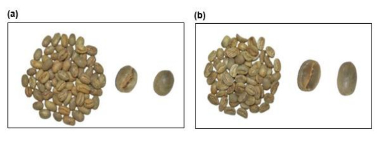
Peaberries are a special type of coffee bean with an oval shape. Peaberries are not considered defective, but separating peaberries is important to make the shapes of the remaining beans uniform for roasting evenly. The separation of peaberries and normal coffee beans increases the value of both peaberries and normal coffee beans in the market. However, it is difficult to sort peaberries from normal beans using existing commercial sorting machines because of their similarities. In previous studies, we have shown the availability of image processing and machine learning techniques, such as convolutional neural networks (CNNs), support vector machines (SVMs), and k-nearest-neighbors (KNNs), for the classification of peaberries and normal beans using a powerful desktop PC. As the next step, assuming the use of our system in the least developed countries, this study was performed to examine their implementation in and the limitations of Raspberry Pi 3. To improve the performance, we modified the CNN architecture from our previous studies. As a result, we found that the CNN model outperformed both linear SVM and KNN on the use of Raspberry Pi 3. For instance, the trained CNN could classify approximately 13.77 coffee bean images per second with 98.19% accuracy of the classification with 64×64 pixel color images on Raspberry Pi 3. There were limitations of Raspberry Pi 3 for linear SVM and KNN on the use of large image sizes because of the system's small RAM size. Generally, the linear SVM and KNN were faster than the CNN with small image sizes, but we could not obtain better results with both the linear SVM and KNN than the CNN in terms of the classification accuracy. Our results suggest that the combination of the CNN and Raspberry Pi 3 holds the promise of inexpensive peaberries and a normal bean sorting system for the least developed countries.
- Convolutional Neural Networks (CNN),
- coffee bean,
- K-Nearest-Neighbors (KNN),
- peaberry,
- Raspberry Pi 3,
- Support Vector Machine (SVM)
Citation: Hira Lal Gope, Hidekazu Fukai. Peaberry and normal coffee bean classification using CNN, SVM, and KNN: Their implementation in and the limitations of Raspberry Pi 3[J]. AIMS Agriculture and Food, 2022, 7(1): 149-167. doi: 10.3934/agrfood.2022010

Related Papers:

Abstract

Peaberries are a special type of coffee bean with an oval shape. Peaberries are not considered defective, but separating peaberries is important to make the shapes of the remaining beans uniform for roasting evenly. The separation of peaberries and normal coffee beans increases the value of both peaberries and normal coffee beans in the market. However, it is difficult to sort peaberries from normal beans using existing commercial sorting machines because of their similarities. In previous studies, we have shown the availability of image processing and machine learning techniques, such as convolutional neural networks (CNNs), support vector machines (SVMs), and k-nearest-neighbors (KNNs), for the classification of peaberries and normal beans using a powerful desktop PC. As the next step, assuming the use of our system in the least developed countries, this study was performed to examine their implementation in and the limitations of Raspberry Pi 3. To improve the performance, we modified the CNN architecture from our previous studies. As a result, we found that the CNN model outperformed both linear SVM and KNN on the use of Raspberry Pi 3. For instance, the trained CNN could classify approximately 13.77 coffee bean images per second with 98.19% accuracy of the classification with 64×64 pixel color images on Raspberry Pi 3. There were limitations of Raspberry Pi 3 for linear SVM and KNN on the use of large image sizes because of the system's small RAM size. Generally, the linear SVM and KNN were faster than the CNN with small image sizes, but we could not obtain better results with both the linear SVM and KNN than the CNN in terms of the classification accuracy. Our results suggest that the combination of the CNN and Raspberry Pi 3 holds the promise of inexpensive peaberries and a normal bean sorting system for the least developed countries.

References

[1]	Bhumiratana N, Adhikari K, Chambers-Ⅳ E (2011) Evolution of sensory aroma attributes from coffee beans to brewed coffee. LWT-Food Sci Technol 44: 2185–2192. https://doi.org/10.1016/j.lwt.2011.07.001 doi: 10.1016/j.lwt.2011.07.001
[2]	Giacalone D, Degn TK, Yang N, et al. (2019) Common roasting defects in coffee: Aroma composition, sensory characterization and consumer perception. Food Qual Preference 71: 463–474. https://doi.org/10.1016/j.foodqual.2018.03.009 doi: 10.1016/j.foodqual.2018.03.009
[3]	Suhandy D, Yulia M (2017) Peaberry coffee discrimination using UV-visible spectroscopy combined with SIMCA and PLS-DA. Int J Food Prop 20: S331–S339. https://doi.org/10.1080/10942912.2017.1296861 doi: 10.1080/10942912.2017.1296861
[4]	Duarte SMDS, Abreu CMPD, Menezes HCD, et al. (2005) Effect of processing and roasting on the antioxidant activity of coffee brews. Food Sci Technol 25: 387–393. https://doi.org/10.1590/s0101-20612005000200035 doi: 10.1590/s0101-20612005000200035
[5]	Peaberry seed (2020) Available from: https://coffeebrat.com/peaberry-coffee.
[6]	Evolution (2019) Available from: http://blogs.rochester.edu/EEB/?m=geneazyt&paged=42.
[7]	Suhandy D, Yulia M, Kusumiyati (2018) Chemometric quantification of peaberry coffee in blends using UV–visible spectroscopy and partial least squares regression. In: AIP Conference Proceedings, AIP Publishing LLC, 060010. https://doi.org/10.1063/1.5062774
[8]	Peaberry coffee (2020) Available from: https://coffee-brewing-methods.com/coffee-beans-review/peaberry-coffee.
[9]	Fukai H, Furukawa J, Katsuragawa H, et al. (2018) Classification of green coffee beans by convolutional neural network and its implementation on raspberry Pi and Camera Module. Timorese Acad J Sci Technol 1: 10. http://fect.untl.edu.tl/file_tajst/Classification of Green Coffee Beans by Convolutional Neural Network and its Implemnentation on Rasperry and Camera Module.pdf
[10]	Rangarajan AK, Purushothaman R, Ramesh A (2018) Tomato crop disease classification using pre-trained deep learning algorithm. Procedia Comput Sci 133: 1040–1047. https://doi.org/10.1016/j.procs.2018.07.070 doi: 10.1016/j.procs.2018.07.070
[11]	Jahanbakhshi A, Kheiralipour K (2020) Evaluation of image processing technique and discriminant analysis methods in postharvest processing of carrot fruit. Food Sci Nutr 8: 3346–3352. https://doi.org/10.1002/fsn3.1614 doi: 10.1002/fsn3.1614
[12]	Peña JM, Gutiérrez PA, Hervás-Martínez C, et al. (2014) Object-based image classification of summer crops with machine learning methods. Remote Sens 6: 5019–5041. https://doi.org/10.3390/rs6065019 doi: 10.3390/rs6065019
[13]	Pinto C, Furukawa J, Fukai H, et al. (2017) Classification of Green coffee bean images basec on defect types using convolutional neural network (CNN). In: 2017 International Conference on Advanced Informatics, Concepts, Theory, and Applications (ICAICTA), 1–5. https://doi.org/10.1109/ICAICTA.2017.8090980
[14]	Gope HL, Fukai H (2020) Normal and peaberry coffee beans classification from green coffee bean images using convolutional neural networks and support vector machine. Int J Comput Inf Eng 14: 189–196. https://publications.waset.org/10011255/pdf
[15]	Peaberry bean (2019) Available from: http://www.zecuppa.com/coffeeterms-bean-defects.htm.
[16]	Peaberry (2020) Available from: https://gamblebaycoffee.com/peaberry-coffee-beans-better-regular.
[17]	LeCun Y, Bottou L, Bengio Y, et al. (1998) Gradient-based learning applied to document recognition. Proc IEEE 86: 2278–2324. https://doi.org/10.1109/5.726791 doi: 10.1109/5.726791
[18]	LeCun Y, Bengio Y, Hinton G (2015) Deep learning. Nature 521: 436–444. https://doi.org/10.1038/nature14539 doi: 10.1038/nature14539
[19]	Deep learning (2020) Available from: https://mila.quebec/en/publication/deep-learning.
[20]	Sameen MI, Pradhan B (2017) Severity prediction of traffic accidents with recurrent neural networks. Appl Sci 7: 476. https://doi.org/10.3390/app7060476 doi: 10.3390/app7060476
[21]	Butt MA, Khattak AM, Shafique S, et al. (2021) Convolutional neural network based vehicle classification in adverse illuminous conditions for intelligent transportation systems. Complexity 2021: 6644861. https://doi.org/10.1155/2021/6644861 doi: 10.1155/2021/6644861
[22]	Srivastava N, Hinton G, Krizhevsky A, et al. (2014) Dropout: A simple way to prevent neural networks from overfitting. J Mach Learn Res 15: 1929–1958. https://jmlr.org/papers/volume15/srivastava14a/srivastava14a.pdf
[23]	Karen S, Andrew Z (2015) Very deep convolutional networks for large-scale image recognition. Published as a conference paper at ICLR 2015. https://arXiv.org/pdf/1409.1556.pdf%E3%80%82
[24]	Igual L, Seguí S (2017) Introduction to Data Science: A Python Approach to Concepts, Techniques and Applications, Springer, 1–218. https://www.springer.com/gp/book/9783319500164
[25]	Schölkopf B, Smola AJ, Bach F (2001) Learning with kernels: Support vector machines, regularization, optimization, and beyond, MIT press. https://ieeexplore.ieee.org/book/6267332
[26]	Mucherino A, Papajorgji PJ, Pardalos PM (2009) K-nearest neighbor classification. In: Data mining in agriculture, 83–106. https://link.springer.com/chapter/10.1007/978-0-387-88615-2_4
[27]	Danil M, Efendi S, Sembiring RW (2019) The analysis of attribution reduction of K-Nearest Neighbor (KNN) algorithm by using Chi-Square. In: Journal of Physics: Conference Series, IOP Publishing, 012004. https://doi.org/10.1088/1742-6596/1424/1/012004
[28]	Gauswami MH, Trivedi KR (2018) Implementation of machine learning for gender detection using CNN on raspberry Pi platform. In: 2018 2nd International Conference on Inventive Systems and Control (ICISC), IEEE, 608613. https://doi.org/10.1109/ICISC.2018.8398872
[29]	Raspberry Pi (2020) Available from: https://www.raspberrypi.org.
[30]	Raspberry Pi 3 Model B (2020) Available from: https://github.com/ianburkeixiv/Raspberry-Pi-Gesture-App.
[31]	Son TT, Lee C, Le-Minh H, et al. (2020) An evaluation of image-based malware classification using machine learning. In: Hernes M, Wojtkiewicz K, Szczerbicki E, (Eds.) ICCCI 2020: Advances in Computational Collective Intelligence, Communications in Computer and Information Science 1287: 125–138. https://doi.org/10.1007/978-3-030-63119-2_11
[32]	Susanibar G, Ramirez J, Sanchez J, et al. (2021) Development of an automated machine for green coffee beans classification by size and defects. J Adv Agric Technol 8: 17–24. https://doi.org/10.18178/joaat.8.1.17-24 doi: 10.18178/joaat.8.1.17-24

Author Bio: Hira Lal Gope completed the B.Sc. (Honors) and M.S. Engineering (Thesis) in Computer Science and Engineering from the University of Chittagong, Chittagong-4331, Bangladesh, in 2012 and 2017, respectively. He is currently pursuing a PhD degree in informatics with Gifu University from 2019. He started his career in the teaching and research profession as a faculty member at the Sylhet Agricultural University, Sylhet-3100, Bangladesh since 01 January 2013. His main areas of research interest are machine learning, image processing, and data mining. Mr. Gope is an associate member of the Bangladesh Computer Society (BCS).

Reader Comments

Your name:*

Email:*
© 2022 the Author(s), licensee AIMS Press. This is an open access article distributed under the terms of the Creative Commons Attribution License (http://creativecommons.org/licenses/by/4.0)