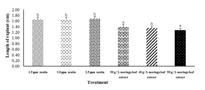
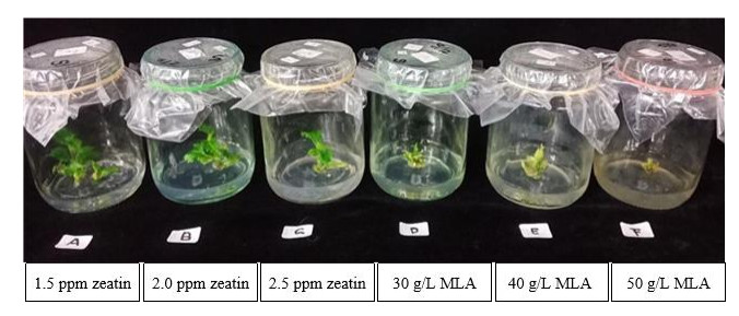
Patchouli is one of the essential oil-producing plants which is commonly found in Indonesia, but the productivity tends to decline. Tissue culture technology is one alternative to increase patchouli plant productivity. Tissue culture requires growth regulators in order for the plants to grow optimally. Moringa plants have the potential as a source of growth regulators for tissue culture because Moringa leaves contain the zeatin hormone. Therefore, a comparison test of various concentrations of the zeatin and the moringa leaf extract is needed to determine whether the Moringa leaf extract can be an alternative to the zeatin hormone. This study aimed to investigate the effect of Moringa leaf extract on the growth of patchouli bud explants. The study employed a complete random design (CRD) with the treatment of concentrations of Moringa leaf extract in MS media. Moringa leaf extract was given at 30 grams/L, 40 grams/L, and 50 grams/L, respectively. Meanwhile, the zeatin hormone was given at a concentration of 1.5 ppm, 2 ppm, and 2.5 ppm. Each treatment was repeated four times. Moringa leaves were extracted by maceration method, and patchouli explants were obtained from the 3rd sub-culture of patchouli shoots. From the research results, it can be concluded that (1) the use of Moringa leaf extract can improve the growth of patchouli explants, and (2) the use of 40 grams/L of Moringa leaf extract can be an alternative to substitute the use of 1.5 ppm zeatin hormone.
Citation: Ellis Nihayati, Merynda Wardatun Najah. Comparative assessment of The Effect of Moringa oleifera Leaf Extract (MLE) and Zeatin on invitro Regeneration Response of Pogostemon cablin Bud Explants[J]. AIMS Agriculture and Food, 2021, 6(1): 308-320. doi: 10.3934/agrfood.2021019
Patchouli is one of the essential oil-producing plants which is commonly found in Indonesia, but the productivity tends to decline. Tissue culture technology is one alternative to increase patchouli plant productivity. Tissue culture requires growth regulators in order for the plants to grow optimally. Moringa plants have the potential as a source of growth regulators for tissue culture because Moringa leaves contain the zeatin hormone. Therefore, a comparison test of various concentrations of the zeatin and the moringa leaf extract is needed to determine whether the Moringa leaf extract can be an alternative to the zeatin hormone. This study aimed to investigate the effect of Moringa leaf extract on the growth of patchouli bud explants. The study employed a complete random design (CRD) with the treatment of concentrations of Moringa leaf extract in MS media. Moringa leaf extract was given at 30 grams/L, 40 grams/L, and 50 grams/L, respectively. Meanwhile, the zeatin hormone was given at a concentration of 1.5 ppm, 2 ppm, and 2.5 ppm. Each treatment was repeated four times. Moringa leaves were extracted by maceration method, and patchouli explants were obtained from the 3rd sub-culture of patchouli shoots. From the research results, it can be concluded that (1) the use of Moringa leaf extract can improve the growth of patchouli explants, and (2) the use of 40 grams/L of Moringa leaf extract can be an alternative to substitute the use of 1.5 ppm zeatin hormone.

| [1] | Nuryani Y, Emmyzar W (2006) Budidaya tanaman nilam. Balai Penelit Tanam Rempah Dan Aromat Pus Penelit Dan Pengemb Perkeb Badan Penelit Dan Pengemb Pertan. Available from: http://nad.litbang.pertanian.go.id/ind/images/dokumen/modul/19-Budidaya%20tanaman%20Nilam1.pdf. |
| [2] | Setiawan RR (2013) Produktivitas nilam nasional semakin menurun (45% total areal pertanaman nilam di Indonesia produksinya < 150 kg/ha). Warta Penelitian Pengembangan Tanaman Industri 19: 8-11. Available from: http://perkebunan.litbang.pertanian.go.id/id/produktivitas-nilam-nasional-semakin-menurun/. |
| [3] |
Singh RP, Manchanda G, Maurya IK, et al. (2019) Streptomyces from rotten wheat straw endowed the high plant growth potential traits and agro-active compounds. Biocatal Agric Biotechnol 17: 507-513. doi: 10.1016/j.bcab.2019.01.014

|
| [4] |
Prajakta BM, Suvarna PP, Raghvendra SP, et al. (2019) Potential biocontrol and superlative plant growth promoting activity of indigenous Bacillus mojavensis PB-35 (R11) of soybean (Glycine max) rhizosphere. SN Appl Sci 1: 1143. doi: 10.1007/s42452-019-1149-1
|
| [5] |
Schä;fer M, Brütting C, Meza-Canales ID, et al. (2015) The role of cis-zeatin-type cytokinins in plant growth regulation and mediating responses to environmental interactions. J Exp Bot 66: 4873-4884. doi: 10.1093/jxb/erv214
|
| [6] | Sulis S, Pangesti R (2015) Pengaruh pemberian air tauge dan air kelapa terhadap pertumbuhan tunas nilam (Pogestemon cablin Benth) secara in vitro. STIGMA J Mat Dan Ilmu Pengetah Alam Unipa 8. |
| [7] |
Ružić DV, Vujović T (2008) The effects of cytokinin types and their concentration on in vitro multiplication of sweet cherry cv. Lapins (Prunus avium L.). Hortic Sci 35: 12-21. doi: 10.17221/646-HORTSCI
|
| [8] | Saburu DV, Polii B, Pinaria A, et al. (2016) Pengaruh zeatin terhadap multiplikasi tunas eksplan nodus pada tanaman krisan varietas kulo dan puspita nusantara. COCOS 7: 1-8. |
| [9] |
Peixe A, Raposo A, Lourenço R, et al. (2007) Coconut water and BAP successfully replaced zeatin in olive (Olea europaea L.) micropropagation. Sci Hortic 113: 1-7. doi: 10.1016/j.scienta.2007.01.011
|
| [10] |
Ali EF, Hassan FAS, Elgimabi M (2018) Improving the growth, yield and volatile oil content of Pelargonium graveolens L. Herit by foliar application with moringa leaf extract through motivating physiological and biochemical parameters. South Afr J Bot 119: 383-389. doi: 10.1016/j.sajb.2018.10.003
|
| [11] |
Vongsak B, Sithisarn P, Mangmool S, et al. (2013) Maximizing total phenolics, total flavonoids contents and antioxidant activity of Moringa oleifera leaf extract by the appropriate extraction method. Ind Crops Prod 44: 566-571. doi: 10.1016/j.indcrop.2012.09.021
|
| [12] | Krisnadi A (2015) Kelor Super Nutrisi Edisi Revisi. Available from: https://kelorina.com/ebook.pdf. |
| [13] |
Bholah K, Ramful‐Baboolall D, Neergheen‐Bhujun VS (2015) Antioxidant Activity of Polyphenolic Rich M oringa oleifera L am. Extracts in Food Systems. J Food Biochem 39: 733-741. doi: 10.1111/jfbc.12181
|
| [14] | Anwar F, Latif S, Ashraf M, et al. (2007) Moringa oleifera: a food plant with multiple medicinal uses. Phytother Res: Int J Devoted Pharmacol Toxicol Eval Nat Prod Deriv 21: 17-25. |
| [15] | Ashfaq M, Basra SM, Ashfaq U (2012) Moringa: a miracle plant for agro-forestry. J Agric Soc Sci 8. |
| [16] | Suminar E, Anjarsari IRD, Nuraini A, et al. (2015) Pertumbuhan dan perkembangan tunas nilam var. Lhoukseumawe dari jenis eksplan dengan sitokinin yang berbeda secara in vitro. Kultivasi 14. |
| [17] |
Susilowati A, Listyawati S (2001) Keanekaragaman jenis Mikroorganisme sumber kontaminasi kultur In Vitro di Sub Lab Biologi laboratorium MIPA Pusat UNS. Biodiversitas 2: 110-114. doi: 10.13057/biodiv/d020105
|
| [18] |
Coppin JP, Xu Y, Chen H, et al. (2013) Determination of flavonoids by LC/MS and anti-inflammatory activity in Moringa oleifera. J Funct Foods 5: 1892-1899. doi: 10.1016/j.jff.2013.09.010
|
| [19] |
Singh RG, Negi PS, Radha C (2013) Phenolic composition, antioxidant and antimicrobial activities of free and bound phenolic extracts of Moringa oleifera seed flour. J Funct Foods 5: 1883-1891. doi: 10.1016/j.jff.2013.09.009
|
| [20] |
Rodríguez-Pérez C, Quirantes-Piné R, Fernández-Gutiérrez A, et al. (2015) Optimization of extraction method to obtain a phenolic compounds-rich extract from Moringa oleifera Lam leaves. Ind Crops Prod 66: 246-254. doi: 10.1016/j.indcrop.2015.01.002
|
| [21] |
Singh AK, Rana HK, Tshabalala T, et al. (2020) Phytochemical, nutraceutical and pharmacological attributes of a functional crop Moringa oleifera Lam: An overview. South Afr J Bot 129: 209-220. doi: 10.1016/j.sajb.2019.06.017
|
| [22] | Munggarani M, Suminar E, Nuraini A, et al. (2018) Multiplikasi Tunas Meriklon Kentang Pada Berbagai Jenis dan Konsentrasi Sitokinin. Agrologia 7. |
| [23] | Phiri C, Mbewe DN (2010) Influence of Moringa oleifera leaf extracts on germination and seedling survival of three common legumes. Int J Agric Biol 12: 315-317. |
| [24] | Nouman W, Siddiqui MT, Basra SMA (2012) Moringa oleifera leaf extract: An innovative priming tool for rangeland grasses. Turk J Agric For 36: 65-75. |
| [25] | Yasmeen A, Basra SMA, Wahid A, et al. (2013) Exploring the potential of Moringa oleifera leaf extract (MLE) as a seed priming agent in improving wheat performance. Turk J Bot 37: 512-520. |
| [26] |
Yasmeen A, Nouman W, Basra SMA, et al. (2014) Morphological and physiological response of tomato (Solanumlycopersicum L.) to natural and synthetic cytokinin sources: a comparative study. Acta Physiol Plant 36: 3147-3155. doi: 10.1007/s11738-014-1662-1
|
| [27] | Kasutjianingati RP, Khumaida N, Efendi D (2010) Kemampuan pecah tunas dan kemampuan berbiak mother plant pisang Rajabulu (AAB) dan pisang Tanduk (AAB) dalam medium inisiasi in vitro. Agriplus 20: 39-46. |
| [28] |
Ulvskov P, Nielsen TH, Seiden P, et al. (1992) Cytokinins and leaf development in sweet pepper (Capsicum annuum L.). Planta 188: 70-77. doi: 10.1007/BF01160714
|
| [29] |
Chen JT, Chang C, Chang WC (1999) Direct somatic embryogenesis on leaf explants of Oncidium Gower Ramsey and subsequent plant regeneration. Plant Cell Rep 19: 143-149. doi: 10.1007/s002990050724
|
| [30] |
Chen JT, Chang WC (2001) Effects of auxins and cytokinins on direct somatic embryogenesison leaf explants of Oncidium'Gower Ramsey'. Plant Growth Regul 34: 229-232. doi: 10.1023/A:1013304101647
|
| [31] |
Gajdošová S, Spíchal L, Kamínek M, et al. (2011) Distribution, biological activities, metabolism, and the conceivable function of cis-zeatin-type cytokinins in plants. J Exp Bot 62: 2827-2840. doi: 10.1093/jxb/erq457
|
| [32] |
Rosniawaty S, Anjarsari IRD, Sudirja R (2019) Aplikasi sitokinin untuk meningkatkan pertumbuhan tanaman teh di dataran rendah. Jurnal Tanaman Industri dan Penyegar 5: 31. doi: 10.21082/jtidp.v5n1.2018.p31-38
|
| [33] | Kieber JJ, Schaller GE (2014) Cytokinins. Arab Book: American Soc Plant Biol 12. |
| [34] |
Hwang I, Sheen J, Müller B (2012) Cytokinin signaling networks. Annu Rev Plant Biol 63: 353-380. doi: 10.1146/annurev-arplant-042811-105503
|
| [35] | George EF, Hall MA, De Klerk GJ (2008) Plant growth regulators Ⅱ: cytokinins, their analogues and antagonists. Plant propagation by tissue culture, Springer, 205-226. |
| [36] | Sholikhah EN, Wijayanti MA (2006) In vitro antiplasmodial activity and cytotoxicity of new n-benzyl 1, 10-phenanthroline derivatives. Southeast Asian J Trop Med Public Health 37: 1072-1077. |
| [37] |
Seswita D (2020) Penggunaan air kelapa sebagai zat pengatur tumbuh pada multiplikasi tunas temulawak (Curcuma xanthorrhiza Roxb.) in vitro. Jurnal Penelitian Tanaman Industri 16: 135-140. doi: 10.21082/jlittri.v16n4.2010.135-140
|
| [38] |
Kuraishi S, Muir RM (1964) The relationship of gibberellin and auxin in plant growth. Plant Cell Physiol 5: 61-69. doi: 10.1093/oxfordjournals.pcp.a079024
|
| [39] |
Ockerse R, Galston AW (1967) Gibberellin-auxin interaction in pea stem elongation. Plant Physiol 42: 47-54. doi: 10.1104/pp.42.1.47
|
| [40] | Dalessandro G (1973) Interaction of auxin, cytokinin, and gibberellin on cell division and xylem differentiation in cultured explants of Jerusalem artichoke. Plant Cell Physiol 14: 1167-1176. |
| [41] | Kazama H, Katsumi M (1973) Auxin-gibberellin relationships in their effects on hypocotyl elongation of light-grown cucumber seedlings. Responses of sections to auxin, gibberellin and sucrose. Plant Cell Physiol 14: 449-458. |
| [42] | Ross JJ, O'neill DP, Wolbang CM, et al. (2001) Auxin-gibberellin interactions and their role in plant growth. J Plant Growth Regul 20: 336-353. |
| [43] |
Ross JJ, O'Neill DP, Rathbone DA (2003) Auxin-gibberellin interactions in pea: integrating the old with the new. J Plant Growth Regul 22: 99-108. doi: 10.1007/s00344-003-0021-z
|
| [44] |
DeMason DA (2005) Auxin-cytokinin and auxin-gibberellin interactions during morphogenesis of the compound leaves of pea (Pisum sativum). Planta 222: 151-166. doi: 10.1007/s00425-005-1508-6
|
| [45] | Gbadamosi IT, Sulaiman MO (2012) The Influence of Growth Hormones and Cocos nucifera Water on the In Vitro Propagation of Irvingia gabonensis (Aubry-Lecomte ex O'Rorke) Baill. Nat Sci 10: 53-58. |
| [46] |
de Souza RAV, Braga FT, Setotaw TA, et al. (2013) Effect of coconut water on growth of olive embryos cultured in vitro. Ciênc Rural 43: 290-296. doi: 10.1590/S0103-84782013000200016
|
| [47] |
Muhammad K, Gul Z, Jamal Z, et al. (2015) Effect of coconut water from different fruit maturity stages, as natural substitute for synthetic PGR in in vitro potato micropropagation. Int J Biosci IJB 6: 84-92. doi: 10.12692/ijb/6.2.84-92
|
| [48] |
Demason DA, Chawla R (2006) Auxin/gibberellin interactions in pea leaf morphogenesis. Bot J Linn Soc 150: 45-59. doi: 10.1111/j.1095-8339.2006.00491.x
|
| [49] |
Ferreira PMP, Farias DF, Oliveira JT de A, et al. (2008) Moringa oleifera: bioactive compounds and nutritional potential. Rev Nutr 21: 431-437. doi: 10.1590/S1415-52732008000400007
|
| [50] |
Moyo B, Masika PJ, Hugo A, et al. (2011) Nutritional characterization of Moringa (Moringa oleifera Lam.) leaves. Afr J Biotechnol 10: 12925-12933. doi: 10.5897/AJB10.1599
|
| [51] | Madukwe EU, Ezeugwu JO, Eme PE (2013) Nutrient composition and sensory evaluation of dry Moringa oleifera aqueous extract. Corpus ID: 10868940. |

Figures(4) / Tables(2)

Ellis Nihayati, Merynda Wardatun Najah. Comparative assessment of The Effect of Moringa oleifera Leaf Extract (MLE) and Zeatin on invitro Regeneration Response of Pogostemon cablin Bud Explants[J]. AIMS Agriculture and Food, 2021, 6(1): 308-320. doi: 10.3934/agrfood.2021019


 DownLoad: