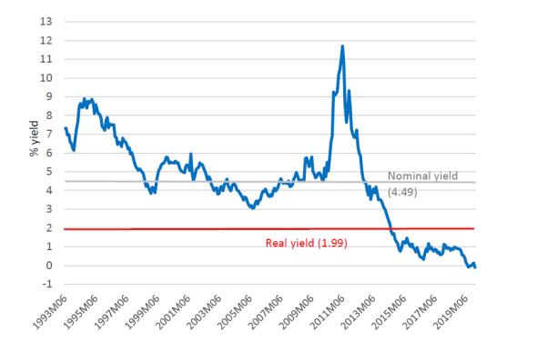
The global practice of Cost-Benefit Analysis (CBA), to analyse the welfare impacts of public investments, has undergone profound changes in recent years. The reforms in general practice have primarily been driven by the discussions of the implications of climate change and environmental degradation. Central to the discussion has been the social discount rate, used to value future costs and benefits in the present, and also the dual discount rates for "environmental goods", as goods that are of no, or of risky substitution. Official rates, in many nations, are calculated using the "Ramsey" formula. The literature has explored the relevant factors in this formula, but with less attention paid to the selection of the rate of future growth in consumption, or to the setting of dual discount rates in national practice guidance. Through considering the case of Ireland, this study demonstrates that the selection of growth rates in consumption, in the context of future uncertainty, requires the use of plausible scenarios, rather than historical trends or forecasts. By employing economic scenarios, alongside established values for the other factors, the main discount rate for Ireland is calculated in a range of 1.7 to 2.8 per cent. Seperately, a dual discount rate, for capital that cannot be replaced, is estimated at ≤1.3 per cent. The main discount rate is validated by comparison against discount rates found in the literature, applied in other comparable nations, and by the rate estimated from the real yield on government bonds. All four independent lines of evidence support the range estimated. This demonstrates that the Irish government's estimated discount rate, of 4.0 per cent, is not credible, and needs reduction, alongside introduction of dual discounting.
Citation: Tadhg O'Mahony. Cost-benefit analysis in a climate of change: setting social discount rates in the case of Ireland[J]. Green Finance, 2021, 3(2): 175-197. doi: 10.3934/GF.2021010
The global practice of Cost-Benefit Analysis (CBA), to analyse the welfare impacts of public investments, has undergone profound changes in recent years. The reforms in general practice have primarily been driven by the discussions of the implications of climate change and environmental degradation. Central to the discussion has been the social discount rate, used to value future costs and benefits in the present, and also the dual discount rates for "environmental goods", as goods that are of no, or of risky substitution. Official rates, in many nations, are calculated using the "Ramsey" formula. The literature has explored the relevant factors in this formula, but with less attention paid to the selection of the rate of future growth in consumption, or to the setting of dual discount rates in national practice guidance. Through considering the case of Ireland, this study demonstrates that the selection of growth rates in consumption, in the context of future uncertainty, requires the use of plausible scenarios, rather than historical trends or forecasts. By employing economic scenarios, alongside established values for the other factors, the main discount rate for Ireland is calculated in a range of 1.7 to 2.8 per cent. Seperately, a dual discount rate, for capital that cannot be replaced, is estimated at ≤1.3 per cent. The main discount rate is validated by comparison against discount rates found in the literature, applied in other comparable nations, and by the rate estimated from the real yield on government bonds. All four independent lines of evidence support the range estimated. This demonstrates that the Irish government's estimated discount rate, of 4.0 per cent, is not credible, and needs reduction, alongside introduction of dual discounting.

| [1] | ADB (2009) Cost-Benefit Analysis for Development: a Practical Guide. Asian Development Bank, Manila. |
| [2] | Barker T (2008) The economics of avoiding dangerous climate change. An editorial essay on The Stern Review. Clim Change 89: 173-194. |
| [3] |
Baumgartner S, Klein AM, Thiel D, et al. (2015) Ramsey discounting of ecosystem services. Environ Resour Econ 61: 273-296. doi: 10.1007/s10640-014-9792-x

|
| [4] |
Baumstark L, Gollier C, (2014) The relevance and the limits of the Arrow-Lind Theorem. J Natural Resour Policy Res 6: 45-49. doi: 10.1080/19390459.2013.861160
|
| [5] | Beckerman W, Hepburn C (2007) Ethics of the discount rate in the Stern Review on the Economics of Climate Change. World Econ 8: 187-210. |
| [6] | Bergin A, Morgenroth E, McQuinn K (2016) Ireland's Economic Outlook: Perspectives and Policy Challenges. Available from: http://www.esri.ie/pubs/EO1.pdf. |
| [7] |
Boardman AE, Moore MA, Vining AR (2010) The social discount rate for Canada based on future growth in consumption. Can Public Policy 36: 325-343. doi: 10.3138/cpp.36.3.325
|
| [8] | Chua AJ, Choong WW (2016) A Review of Approaches to Construct Social Discount Rate. Sains Humanika 8: 37-42. |
| [9] | Council of Economic Advisers (2017) Discounting for Public Policy: Theory and Recent Evidence on the Merits of Updating the Discount Rate. Council of Economic Advisers Issue Brief January 2017. Available from: https://obamawhitehouse.archives.gov/sites/default/files/page/files/20170 1_cea_discounting_issue_brief.pdf. |
| [10] | CSO (2020) FIM08: Financial Interest Rates by Interest Rate and Month Available from: https://www.cso.ie/px/pxeirestat/Statire/SelectVarVal/Define.asp?maintable=FIM08&PLanguage=0. |
| [11] | Daneshmand A, Jahangard E, Abdollah‑Milani M (2018) A time preference measure of the social discount rate for Iran. Econ Struct 7: 29. |
| [12] |
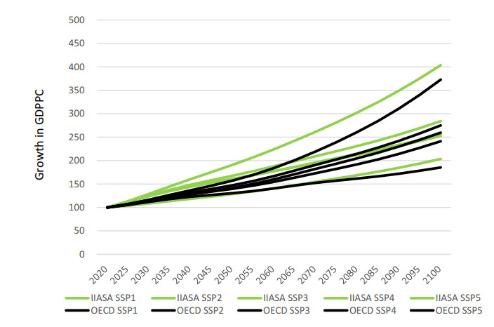
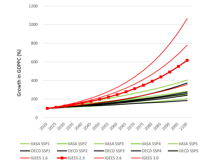
Dellink R, Chateau J, Lanzi E, et al. (2017) Long-term economic growth projections in the Shared Socioeconomic Pathways. Global Environ Change 42: 200-214. doi: 10.1016/j.gloenvcha.2015.06.004
|
| [13] | DPER (2012) The Public Spending Code D. Standard Analytical Procedures Guide to economic appraisal: Carrying out a cost benefit analysis D.03. Department of Public Expenditure and Reform. Available from: http://publicspendingcode.per.gov.ie/wpcontent/uploads/2012/08/D03-Guide-to-economic-appraisal-CBA-16-July.pdf. |
| [14] | DPER (2019) Circular 18/2019: Update of the Public Spending Code (PSC): Central Technical References and Economic Appraisal Parameters. Department of Public Expenditure and Reform. Available from: https://assets.gov.ie/20001/35c13bbd055a4a09961a4ec59c93c798.pdf. |
| [15] | DGECFIN (2017) The 2018 Ageing Report, Underlying Assumptions & Projection Methodologies. Directorate for Economic and Financial Affairs. Available from: https://ec.europa.eu/info/sites/info/files/economy-finance/ip065_en.pdf. |
| [16] |
Drupp MA, Freeman MC, Groom B, et al. (2018) Discounting disentangled. Am Econ J Econ Policy 10: 109-134. doi: 10.1257/pol.20160240
|
| [17] | Drupp MA (2016) Limits to substitution between ecosystem services and manufactured goods and implications for social discounting. Environ Resour Econ 69: 135-158. |
| [18] | European Commission (2016) Better Regulation Toolbox. Available from: https://ec.europa.eu/info/law/law-making-process/planning-and-proposing-law/better-regulation -why-and-how/better-regulation-guidelines-and-toolbox_en. |
| [19] | EEA (2015) The European Environment: State and Outlook 2015. Copenhagen: European Environment Agency. Available from: http://www.eea.europa.eu/soer. |
| [20] |
Evans, D (2005) The Elasticity of Marginal Utility of Consumption: Estimates for 20 OECD Countries. Fiscal Stud 26: 197-224. doi: 10.1111/j.1475-5890.2005.00010.x
|
| [21] |
Evans D, Sezer H (2004) Social Discount Rates for Six Major Countries. Appl Econ Lett 11: 557-560. doi: 10.1080/135048504200028007
|
| [22] | Fleurbaey M, Kartha S, Bolwig S, et al. (2014) Sustainable Development and Equity, In: Climate Change 2014: Mitigation of Climate Change, Contribution of Working Group III to the Fifth Assessment Report of the Intergovernmental Panel on Climate Change, Edenhofer O, Pichs-Madruga R, Sokona Y, Farahani E, Kadner S, Seyboth K, Adler A, Baum I, Brunner S, Eickemeier P, Kriemann B, Savolainen J, Schlömer S, von Stechow C, Zwickel T and Minx JC, (eds.), Cambridge University Press, Cambridge, United Kingdom and New York, NY, USA. |
| [23] |
Frankel J (2011) Over-optimism in forecasts by official budget agencies and its implications. Oxford Rev Econ Policy 27: 536-562. doi: 10.1093/oxrep/grr025
|
| [24] | Freeman M, Groom B, Spackman M (2018) Social Discount Rates for Cost-Benefit Analysis: A Report for HM Treasury. Available from: https://assets.publishing.service.gov.uk/government/uploads/ system/uploads/attachment_data/file/685904/Social_Discount_Rates_for_Cost-Benefit_ Analysis_A_Report_for_HM_Treasury.pdf. |
| [25] | Gollier C (2011) Le calcul du risque dans les investissements publics, Centre d'Analyse Stratégique, Rapports & Documents n°36, La Documentation Franç aise. Available from: http://archives.strategie.gouv.fr/cas/system/files/rapport_36_diffusion.pdf. |
| [26] |
Halicioglu F, Karatas C (2013) A social discount rate for Turkey. Qual Quant 47: 1085-1091. doi: 10.1007/s11135-011-9585-z
|
| [27] | Hartwick JM (1977) Intergenerational Equity and the Investment of Rents from Exhaustible Resources. Am Econ Rev 67: 972-974. |
| [28] | Treasury HM (2003) The Green Book. Appraisal and Evaluation in Central Government. Available from: http://www.fao.org/ag/humannutrition/33236-040551a7cfbc0e73909932192db580c4.pdf. |
| [29] | Treasury HM (2018) The Green Book. Central Government Guidance on Appraisal and Evaluation. Available from: https://assets.publishing.service.gov.uk/government/uploads/system/uploads/ attachment_data/file/685903/The_Green_Book.pdf. |
| [30] | Hulme M (2009) Why We Disagree About Climate Change: Understanding Controversy, Inaction and Opportunity, Cambridge, UK: Cambridge University Press. |
| [31] | IGEES (2018) Central Technical Appraisal ParametersDiscount Rate, Time Horizon, Shadow Price of Public Funds and Shadow Price of Labour. Available from: https://igees.gov.ie/wp-content/uploads/2019/07/Parameters-Paper-Final-Version.pdf. |
| [32] | IPBES (2019) Summary for policymakers of the global assessment report on biodiversity and ecosystem services of the Intergovernmental Science-Policy Platform on Biodiversity and Ecosystem Services, Díaz S, Settele J, Brondízio ES, Ngo HT, Guèze M, Agard J, Arneth A, Balvanera P, Brauman KA, Butchart SHM, Chan KMA, Garibaldi LA, Ichii K, Liu J, Subramanian SM, Midgley GF, Miloslavich P, Molnár Z, Obura D, Pfaff A, Polasky S, Purvis A, Razzaque J, Reyers B, Roy Chowdhury R, Shin YJ, Visseren-Hamakers IJ, Willis KJ, and Zayas CN, (eds.), IPBES secretariat, Bonn, Germany, 56. |
| [33] | IPCC (2014) Climate Change 2014: Synthesis Report, Contribution of Working Groups I, II and III to the Fifth Assessment Report of the Intergovernmental Panel on Climate Change, Core Writing Team, Pachauri RK and Meyer LA (eds.), IPCC, Geneva, Switzerland, 151. |
| [34] | IPCC (2018) Global warming of 1.5℃. An IPCC Special Report on the impacts of global warming of 1.5℃ above pre-industrial levels and related global greenhouse gas emission pathways, in the context of strengthening the global response to the threat of climate change, sustainable development, and efforts to eradicate poverty, Masson-Delmotte V, Zhai P, Pörtner HO, Roberts D, Skea J, Shukla PR, Pirani A, Moufouma-Okia W, Péan C, Pidcock R, Connors S, Matthews JBR, Chen Y, Zhou X, Gomis MI, Lonnoy E, Maycock T, Tignor M, Waterfield T (eds.). |
| [35] | Kolstad C, Urama K, Broome J, et al. (2014) Social, Economic and Ethical Concepts and Methods, In: Climate Change 2014: Mitigation of Climate Change, Contribution of Working Group III to the Fifth Assessment Report of the Intergovern-mental Panel on Climate Change, Edenhofer O, Pichs-Madruga R, Sokona Y, Farahani E, Kadner S, Seyboth K, Adler A, Baum I, Brunner S, Eickemeier P, Kriemann B, Savolainen J, Schlömer S, von Stechow C, Zwickel T and Minx JC (eds.), Cambridge University Press, Cambridge, United Kingdom and New York, NY, USA. |
| [36] |
Kossova T, Sheluntcova M (2016) Evaluating performance of public sector projects in Russia: The choice of a social discount rate. Int J Project Manage 34: 403-411. doi: 10.1016/j.ijproman.2015.11.005
|
| [37] | Kula E (1996) Social project appraisal and historical development of ideas on discounting—a legacy for the 1990's and beyond. Cost-benefit Analysis and Project Appraisal in Developing Countriesedited by Colin H. Kirkpatrick, John Weiss, Elgar. |
| [38] |
Kula E (2004) Estimation of a social rate of interest for India. J Agric Econ 55: 91-99. doi: 10.1111/j.1477-9552.2004.tb00081.x
|
| [39] | Kula E (2008) Economics of Discounting—British experience and lessons to be learned, 2008, Paper presented at the 15th World Congress of the International Economic Association, Istanbul. |
| [40] |
Kula E, Evans D (2011) Dual discounting in cost-benefit analysis for environmental impacts. Environ Impact Assess Rev 31: 180-186. doi: 10.1016/j.eiar.2010.06.001
|
| [41] | Kyllonen S, Basso A (2017) When utility maximization is not enough: intergenerational sufficientarianism and the economics of climate change, Chapter 5, The Ethical Underpinnings of Climate Economics, Routledge. |
| [42] | Lebegue D (2005) Revision du taux d'actualisation des investissements publics, Rapport du groupe de experts, Commisariat Generale de Plan, Paris. Available from: https://www.oieau.org/eaudoc/system/files/documents/44/223176/223176_doc.pdf. |
| [43] |
Leimbach M, Kriegler E, Roming N, et al. (2017) Future growth patterns of world regions—A GDP scenario approach. Global Environ Change 42: 215-225. doi: 10.1016/j.gloenvcha.2015.02.005
|
| [44] | Lopez H (2008) The social discount rate: estimates for nine Latin American countries. The World Bank, Policy Research Working Paper 4639, 17. |
| [45] | Maddison D, Day B (2015) Improving Cost Benefit Analysis Guidance, Natural Capital Committee, London. Millennium Ecosystem Assessment (2005). Ecosystems and Human Well-being: Current State and Trends. Vol. 1. Washington, DC: Island Press. |
| [46] |
Moore M, Boardman A, Vining A (2013) More appropriate discounting: the rate of social time preference and the value of the social discount rate. J Benefit Cost Anal 4: 1-16. doi: 10.1515/jbca-2012-0008
|
| [47] | Morikawa M (2020) Uncertainty in long-term macroeconomic forecasts: Ex post evaluation of forecasts by economics researchers. Q Rev Econ Financ [In Press]. |
| [48] | Organisation for Economic Cooperation and Development (OECD) (2018) Cost-Benefit Analysis and the Environment. Organisation for Economic Cooperation and Development, Paris, France. |
| [49] | Organisation for Economic Cooperation and Development (OECD) (2020) Anticipatory innovation governance: Shaping the future through proactive policy making, OECD Working Papers on Public Governance, No. 44, OECD Publishing, Paris. Available from: https://doi.org/10.1787/cce14d80-en. |
| [50] | O'Mahony T (2018) Appraisal in transition: 21st century challenges and updating Cost-Benefit Analysis in Ireland. Technical Report. |
| [51] | O'Mahony T (2021) Cost-Benefit Analysis and the environment: The time horizon is of the essence. Environ Impact Assess Rev 89: 106587. |
| [52] |
Percoco M (2008) A social discount rate for Italy. Appl Econ Lett15: 73-77. doi: 10.1080/13504850600706537
|
| [53] | Quinet E (2013) L'évaluation socioéconomique des investissements publics, Tome 1 Rapport final, Commissariat Generale a la strategie et a la Prospective, Paris. Available from: www.strategie.gouv.fr/sites/strategie.gouv.fr/files/atoms/files/cgsp_evaluation_socioeconomique_29072014.pdf. |
| [54] |
Ramsey FP (1928) A Mathematical Theory of Saving. Econ J 38: 543-559. doi: 10.2307/2224098
|
| [55] | Regio DG (2008) Guide to Cost-Benefit Analysis of Investment projects. European Commission Directorate General for Regional and Urban Policy. Available from: http://ec.europa.eu/regional_policy/sources/docgener/guides/cost/guide2008_en.pdf. |
| [56] | Sartori D, Catalano G, Genco M, et al. (2014) Guide to Cost-Benefit Analysis of Investment Project: Economic appraisal tool for Cohesion Policy 2014-2020. European Commission Directorate General for Regional and Urban Policy. Available from: http://ec.europa.eu/regional_policy/sources/docgener/studies/pdf/cba_guide.pdf. |
| [57] |
Schad M, John J (2012) Towards a social discount rate for the economic evaluation of health technologies in Germany: an exploratory analysis. Eur J Health Econ 13: 127-144. doi: 10.1007/s10198-010-0292-9
|
| [58] |
Solow RM (1957) Technical Change and the Aggregate Production Function. Rev Econ Stat 39: 312-320. doi: 10.2307/1926047
|
| [59] | Spackman M (2015) Social time discounting: Institutional and analytical perspectives. Available from: http://www.lse.ac.uk/GranthamInstitute/wp-content/uploads/2015/03/Working-Paper-182-Spackman.pdf. |
| [60] | Spackman M (2017) Social discounting: the SOC/STP divide. Centre for Climate Change Economics and Policy Working Paper No. 207. Grantham Research. |
| [61] | Steffen W, Richardson K, Rockström J, et al. (2015) Planetary Boundaries: Guiding Human Development on a Changing Planet. Science, 347. |
| [62] | Stern, N (2007) The Economics of Climate Change: The Stern Review, Cambridge: Cambridge University Press. |
| [63] | Weikard HP, Zhu X (2005) Discounting and Environmental Quality: When should dual rates be used? Econ Model 22: 868-878. |
| [64] |
Weitzman M (1998) Why the Far-Distant Future Should be Discounted at its Lowest Possible Rate. J Environ Econ Manage 36: 201-208. doi: 10.1006/jeem.1998.1052
|
| [65] | WHO (2006) Guidelines for conducting cost-benefit analysis of household energy and health interventions, by Hutton G. and Rehfuess E., World Health Organisation Publication. |
| [66] | Windsor C (2021) The intellectual ideas inside central banks: what's changed or not since the crisis? J Econ Surv 35: 539-565. |
| [67] | World Bank (2021) Inflation, consumer prices (% annual) -Ireland. Available from: https://data.worldbank.org/indicator/FP.CPI.TOTL.ZG?locations=IE. |
Figures(3) / Tables(2)

Tadhg O'Mahony. Cost-benefit analysis in a climate of change: setting social discount rates in the case of Ireland[J]. Green Finance, 2021, 3(2): 175-197. doi: 10.3934/GF.2021010


 DownLoad: