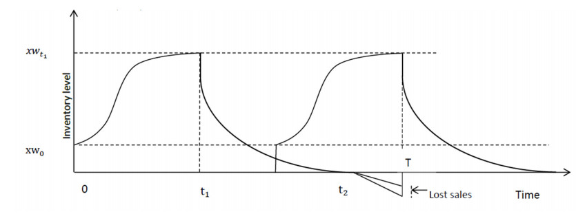
Growing inventory is the set of commodities whose level enhances during the stocking period. This kind of product is normally seen in the poultry industry and livestock farming. In this model, the live newborn is considered to be the initial inventory of the retailer. These are procured and fed until they grow to an ideal weight during the breeding period. Afterward, these are slaughtered and converted to deteriorating items prone to the customer's demand during the consumption period. The poultry industry is responsible for greenhouse gas emissions during feeding, farming, slaughtering, and handling. Consequently, the retailers are enforced to make efforts to reduce the emission which also affects the inventory demeanor. Therefore, the effect of the carbon emissions from the poultry industry has been investigated here. Generally, customers prefer food over the preserved items so shortages are permitted which has been assumed here with partial backlogging. The study has been carried out to investigate the optimum breeding period and optimum livestock inventory. A numerical example and illustrations validate the analytical results. Lastly, a sensitivity analysis has been provided concerning some key parameters.
Citation: Karuna Rana, Shiv Raj Singh, Neha Saxena, Shib Sankar Sana. Growing items inventory model for carbon emission under the permissible delay in payment with partially backlogging[J]. Green Finance, 2021, 3(2): 153-174. doi: 10.3934/GF.2021009
Growing inventory is the set of commodities whose level enhances during the stocking period. This kind of product is normally seen in the poultry industry and livestock farming. In this model, the live newborn is considered to be the initial inventory of the retailer. These are procured and fed until they grow to an ideal weight during the breeding period. Afterward, these are slaughtered and converted to deteriorating items prone to the customer's demand during the consumption period. The poultry industry is responsible for greenhouse gas emissions during feeding, farming, slaughtering, and handling. Consequently, the retailers are enforced to make efforts to reduce the emission which also affects the inventory demeanor. Therefore, the effect of the carbon emissions from the poultry industry has been investigated here. Generally, customers prefer food over the preserved items so shortages are permitted which has been assumed here with partial backlogging. The study has been carried out to investigate the optimum breeding period and optimum livestock inventory. A numerical example and illustrations validate the analytical results. Lastly, a sensitivity analysis has been provided concerning some key parameters.

| [1] |
Cheikhrouhou N, Sarkar B, Malik AI, et al. (2018) Optimization of sample size and order size in an inventory model with quality inspection and return of defective items. Ann Oper Res 271: 445-467. doi: 10.1007/s10479-017-2511-6

|
| [2] |
Donaldson WA (1977) Inventory replenishment policy for a linear trend in demand-an analytical solution. Oper Res Q 28: 663-670. doi: 10.1057/jors.1977.142
|
| [3] |
Dem H, Singh SR (2013) A production model for ameliorating items with quality consideration. Int J Oper Res 17: 183-198. doi: 10.1504/IJOR.2013.053622
|
| [4] |
Goliomytis M, Panopoulou E, Rogdakis E (2003) Growth curves for body weight and major parts, feed consumption and mortality of male broiler chickens raised to maturity. Poultr Sci 82: 1061-1068. doi: 10.1093/ps/82.7.1061
|
| [5] |
Goyal SK (1985) Economic order quantity under conditions of permissible delay in payments. J Oper Res Soc 36: 335-338. doi: 10.1057/jors.1985.56
|
| [6] |
Hollier RH, Mak KL (1983) Inventory replenishment policies for deteriorating items in a declining market. Int J Prod Res 21: 813-826. doi: 10.1080/00207548308942414
|
| [7] |
Hwang H, Shon K (1983) Management of deteriorating inventory under inflation. Eng Econ 28: 191-206. doi: 10.1080/00137918308956072
|
| [8] |
Haley CW, Higgins RC (1973) Inventory policy and trade credit financing. Manage Sci 20: 464-471. doi: 10.1287/mnsc.20.4.464
|
| [9] |
Hua G, Cheng TCE, Wang S (2011) Managing carbon footprints in inventory management. Int J Prod Econ 132: 178-185. doi: 10.1016/j.ijpe.2011.03.024
|
| [10] |
Hu H, Zhou W (2014) A decision support system for joint emission reduction investment and pricing decisions with carbon emission trade. Int J Multimedia Ubiquitous Eng 9: 371-380. doi: 10.14257/ijmue.2014.9.9.37
|
| [11] |
Law ST, Wee HM (2006) An integrated production-inventory model for ameliorating and deteriorating items taking account of time discounting. Math Comput Model 43: 673-685. doi: 10.1016/j.mcm.2005.12.012
|
| [12] |
Mahata GC, De SK (2016) An EOQ inventory system of ameliorating items for price dependent demand rate under retailer partial trade credit policy. Opsearch 53: 889-916. doi: 10.1007/s12597-016-0252-y
|
| [13] |
Moon I, Giri BC, Ko B (2005) Economic order quantity models for ameliorating/deteriorating items under inflation and time discounting. Eur J Oper Res 162: 773-785. doi: 10.1016/j.ejor.2003.09.025
|
| [14] |
Nobil AH, Sedigh AHA, Cardenas-Barron LE (2018) A generalized economic order quantity inventory model with shortage: Case study of a poultry farmer. Arabian J Sci Eng 44: 2653-2663. doi: 10.1007/s13369-018-3322-z
|
| [15] |
Ouyang LY, Wu KS, Yang CT (2006) A study on an inventory model for non-instantaneous deteriorating items with permissible delay in payments. Comp Ind Eng 51: 637-651. doi: 10.1016/j.cie.2006.07.012
|
| [16] |
Pentico DW, Drake MJ (2009) The deterministic EOQ with partial backordering: a new approach. Eur J Oper Res 194: 102-113. doi: 10.1016/j.ejor.2007.12.004
|
| [17] |
Richards F (1959) A flexible growth functions for empirical use. J Exp Botany 10: 290-300. doi: 10.1093/jxb/10.2.290
|
| [18] |
Rezaei J (2014) Economic order quantity for growing items. Int J Prod Econ 155: 109-113. doi: 10.1016/j.ijpe.2013.11.026
|
| [19] | Singh SR, Sharma SA (2016) production reliable model for deteriorating products with random demand and inflation. Int J Syst Sci Oper Logist 4: 330-338. |
| [20] | Singh SR, Singh TJ, Singh C (2007) Perishable inventory model with quadratic demand, partial backlogging and permissible delay in payments. Int Rev Pure Appl Math 3: 199-212. |
| [21] |
Singh SR, Rana K (2020) Effect of inflation and variable holding cost on life time inventory model with multi variable demand and lost sales. Int J Recent Technol Eng 8: 5513–5519. doi: 10.35940/ijrte.E6249.018520
|
| [22] | Singh SR, Rana K (2020) Optimal refill policy for new product and take-back quantity of used product with deteriorating items under inflation and lead time, In: Strategic System Assurance and Business Analytics, 503–515. |
| [23] |
Saxena N, Singh SR, Sana SS (2017) A green supply chain model of vendor and buyer for remanufacturing. RAIRO Oper Res 51: 1133-1150. doi: 10.1051/ro/2016077
|
| [24] |
Singh C, Singh SR (2011) Imperfect production process with exponential demand rate, weibull deterioration under inflation. Int J Oper Res 12: 430-445. doi: 10.1504/IJOR.2011.043551
|
| [25] | Silver EA, Meal HC (1969) A simple modification of the EOQ for the case of a varying demand rate. Prod Inventory Manage 10: 25-65. |
| [26] |
Singh N, Vaish B, Singh SR (2012) An economic production lot-size (EPLS) model with rework flexibility under allowable shortages. Int J Procurement Manage 5: 104-122. doi: 10.1504/IJPM.2012.044156
|
| [27] |
Sarkar B, Majumdar A, Sarkar M, et al. (2018) Effects of variable production rate on quality of products in a single-vendor multi-buyer supply chain management. Int J Adv Manuf Technol 99: 567-581. doi: 10.1007/s00170-018-2527-3
|
| [28] |
Sarkar B, Guchhait R, Sarkar M, et al. (2019) Impact of safety factors and setup time reduction in a two-echelon supply chain management. Robotics Comput-Integrated Manuf 55: 250-258. doi: 10.1016/j.rcim.2018.05.001
|
| [29] |
Sarkar B (2019) Mathematical and analytical approach for the management of defective items in a multi-stage production system. J Clean Prod 218: 896-919. doi: 10.1016/j.jclepro.2019.01.078
|
| [30] |
Taleizadeh AA, Hazarkhani B, Moon I (2020) Joint pricing and inventory decisions with carbon emission considerations, partial backordering and planned discounts. Ann Oper Res 290: 95–113. doi: 10.1007/s10479-018-2968-y
|
| [31] |
Tiwari S, Daryanto Y, Wee HM (2018) Sustainable inventory management with deteriorating and imperfect quality items considering carbon emission. J Clean Prod 192: 281-292. doi: 10.1016/j.jclepro.2018.04.261
|
| [32] |
Turki S, Sauvey C, Rezg N (2018) Modelling and optimization of a manufacturing/remanufacturing system with storage facility under carbon cap and trade policy. J Clean Prod 193: 441–458. doi: 10.1016/j.jclepro.2018.05.057
|
| [33] |
Wee HM, Lo ST, Yu J, et al. (2008) An inventory model for ameliorating and deteriorating itemstaking account of time value of money and finite planning horizon. Int J Syst Sci 39: 801-807. doi: 10.1080/00207720801902523
|
| [34] | Zhang Y, Li L, Tian X, et al. (2016) Inventory management research for growing items with carbon-constrained. Chinese Control Conference, 9588-9593. |
| [35] |
Składanowska-Baryza J, Stanisz M (2019) Pre-slaughter handling implications on rabbit carcass and meat quality-A review. Ann Animal Sci 19: 875-885. doi: 10.2478/aoas-2019-0041
|
| [36] |
Polidori P, Pucciarelli S, Cammertoni N, et al. (2017) The effects of slaughter age on carcass and meat quality of Fabrianese lambs. Small Ruminant Res 155: 12-15. doi: 10.1016/j.smallrumres.2017.08.012
|
| [37] |
Tullo E, Finzi A, Guarino M (2019) Environmental impact of livestock farming and Precision Livestock Farming as a mitigation strategy. Sci Total Environ 650: 2751-2760. doi: 10.1016/j.scitotenv.2018.10.018
|
| [38] |
Tiwari S, Ahmed W, Sarkar B (2018) Multi-item sustainable green production system under trade-credit and partial backordering. J Clean Prod 204: 82–95. doi: 10.1016/j.jclepro.2018.08.181
|

Figures(16) / Tables(2)

Karuna Rana, Shiv Raj Singh, Neha Saxena, Shib Sankar Sana. Growing items inventory model for carbon emission under the permissible delay in payment with partially backlogging[J]. Green Finance, 2021, 3(2): 153-174. doi: 10.3934/GF.2021009


 DownLoad: