To meet the future energy and climate targets in 2030 and 2050 in Austria, it is absolutely necessary to apply extensive measures to reduce the use of fossil fuels. By then, Austria will have to realize a 36% decrease (from 2005 levels) for emission sources outside the European Emission Trading System. The transport sector is a key driver of recently increasing greenhouse gas emissions in Austria. Hence, we examine the macroeconomic and ecologic impacts of an environmental tax reform in Austria from 2020 to 2030. We implement a revenue-neutral tax reform that raises revenues via an increase of the mineral oil tax on diesel and petrol consumption and redistributes these fiscal revenues to the industry and households. In addition, increased fossil fuel taxing would enhance revenues for green investments in e-mobility and thermal refurbishment that stimulate the Austrian economy. The simulation analyses focus on central macroeconomic variables as gross domestic product, employment, investment and private consumption and carbon dioxide emissions. We find that the proposed environmental tax reform generates a triple dividend, leading simultaneously to economic growth and the reduction of greenhouse gas emissions while low-income households can be fully compensated.
Citation: Sebastian Goers, Friedrich Schneider. Economic, ecological and social benefits through redistributing revenues from increased mineral oil taxation in Austria: A triple dividend[J]. Green Finance, 2019, 1(4): 442-456. doi: 10.3934/GF.2019.4.442
Related Papers:
[1]
Feezan Ahmad, Xiao-Wei Tang, Mahmood Ahmad, Roberto Alonso González-Lezcano, Ali Majdi, Mohamed Moafak Arbili .
Stability risk assessment of slopes using logistic model tree based on updated case histories. Mathematical Biosciences and Engineering, 2023, 20(12): 21229-21245.
doi: 10.3934/mbe.2023939
[2]
Sidra Abid Syed, Munaf Rashid, Samreen Hussain, Anoshia Imtiaz, Hamnah Abid, Hira Zahid .
Inter classifier comparison to detect voice pathologies. Mathematical Biosciences and Engineering, 2021, 18(3): 2258-2273.
doi: 10.3934/mbe.2021114
[3]
Liangyu Yang, Tianyu Shi, Jidong Lv, Yan Liu, Yakang Dai, Ling Zou .
A multi-feature fusion decoding study for unilateral upper-limb fine motor imagery. Mathematical Biosciences and Engineering, 2023, 20(2): 2482-2500.
doi: 10.3934/mbe.2023116
[4]
Wajid Aziz, Lal Hussain, Ishtiaq Rasool Khan, Jalal S. Alowibdi, Monagi H. Alkinani .
Machine learning based classification of normal, slow and fast walking by extracting multimodal features from stride interval time series. Mathematical Biosciences and Engineering, 2021, 18(1): 495-517.
doi: 10.3934/mbe.2021027
[5]
Mahmood Ahmad, Feezan Ahmad, Jiandong Huang, Muhammad Junaid Iqbal, Muhammad Safdar, Nima Pirhadi .
Probabilistic evaluation of CPT-based seismic soil liquefaction potential: towards the integration of interpretive structural modeling and bayesian belief network. Mathematical Biosciences and Engineering, 2021, 18(6): 9233-9252.
doi: 10.3934/mbe.2021454
[6]
Lal Hussain, Wajid Aziz, Ishtiaq Rasool Khan, Monagi H. Alkinani, Jalal S. Alowibdi .
Machine learning based congestive heart failure detection using feature importance ranking of multimodal features. Mathematical Biosciences and Engineering, 2021, 18(1): 69-91.
doi: 10.3934/mbe.2021004
[7]
Yanpei Liu, Yunjing Zhu, Yanru Bin, Ningning Chen .
Resources allocation optimization algorithm based on the comprehensive utility in edge computing applications. Mathematical Biosciences and Engineering, 2022, 19(9): 9147-9167.
doi: 10.3934/mbe.2022425
[8]
Natalya Shakhovska, Vitaliy Yakovyna, Valentyna Chopyak .
A new hybrid ensemble machine-learning model for severity risk assessment and post-COVID prediction system. Mathematical Biosciences and Engineering, 2022, 19(6): 6102-6123.
doi: 10.3934/mbe.2022285
[9]
Desire Ngabo, Wang Dong, Ebuka Ibeke, Celestine Iwendi, Emmanuel Masabo .
Tackling pandemics in smart cities using machine learning architecture. Mathematical Biosciences and Engineering, 2021, 18(6): 8444-8461.
doi: 10.3934/mbe.2021418
[10]
Abdulwahab Ali Almazroi .
Survival prediction among heart patients using machine learning techniques. Mathematical Biosciences and Engineering, 2022, 19(1): 134-145.
doi: 10.3934/mbe.2022007
Abstract
To meet the future energy and climate targets in 2030 and 2050 in Austria, it is absolutely necessary to apply extensive measures to reduce the use of fossil fuels. By then, Austria will have to realize a 36% decrease (from 2005 levels) for emission sources outside the European Emission Trading System. The transport sector is a key driver of recently increasing greenhouse gas emissions in Austria. Hence, we examine the macroeconomic and ecologic impacts of an environmental tax reform in Austria from 2020 to 2030. We implement a revenue-neutral tax reform that raises revenues via an increase of the mineral oil tax on diesel and petrol consumption and redistributes these fiscal revenues to the industry and households. In addition, increased fossil fuel taxing would enhance revenues for green investments in e-mobility and thermal refurbishment that stimulate the Austrian economy. The simulation analyses focus on central macroeconomic variables as gross domestic product, employment, investment and private consumption and carbon dioxide emissions. We find that the proposed environmental tax reform generates a triple dividend, leading simultaneously to economic growth and the reduction of greenhouse gas emissions while low-income households can be fully compensated.
1.
Introduction
Slope collapses are complicated natural disasters with devastating consequences [1]. Every year, such hazards cause significant damage to public and private property, traffic disruptions, and lives lost [2,3,4]. As a result, slope stability analyses are essential to prevent and mitigate damages, and better tools for slope assessment are desperately needed in the field of civil engineering. The results of the analysis can be used to identify collapse-prone areas. Based on this data, government agencies can gain a better understanding of slope failure occurrences, and the task of providing financial resources to build retaining structures and developing evacuation plans can be completed more efficiently [2].
The accurate prediction of a rock or soil slope's stability is a difficult problem, owing to the slope's dependency on multiple parameters and the difficulty in determining these values [5]. The term factor of safety (FoS), is commonly used to describe the stability of slopes. FoS is calculated by dividing the resisting forces to the driving forces. The FoS is more than one when the resisting forces of a slope are greater than the driving forces; when the resisting forces are less than the driving forces, the FoS is less than one and the slope is unstable.
Slope stability analysis and prediction approaches have been the focus of many researchers. These efforts have led to development of a number of different and sophisticated formulations for determining FoS and also slope design approaches such as limit equilibrium methods (LEM) [6,7,8,9] continuum mechanics-based numerical techniques [10,11,12], methods based on probabilistic methodologies, such as variational and combination methods [13] and numerical approaches have been widely used as traditional methods for studying slope stability in geotechnical problems. Due of its computational time, LEM simulations may become inadequate. In recent years, however, a number of studies have been conducted to create a number of computational intelligence systems for slope stability analysis.
Data mining approaches have recently proved successful in paving the way for many promising opportunities in slope stability [14,15,16,17,18] and other fields of civil engineering [19,20,21,22,23,24,25,26,27,28,29]. Table 1 lists some representative references for data mining applications for slope stability prediction. The majority of these studies investigated slopes subjected to circular-type failure and stability of these slopes based on geotechnical, geometrical and pore-water pressure parameters. In these studies, data mining approaches based on historical data have been used for two purposes: 1) prediction of slope FoS: the output of these models is the FoS, and 2) prediction of SS status: the output of proposed models shows the slope's stability or instability. However soft computing techniques have proved successful in predicting SS; the fact that most of these techniques are black boxes. The novelty of this article is the development of a transparent and understandable model for predicting SS in slopes that have experienced circular mode failure. The TAN-based model overcomes the shortcomings of other soft computing techniques by producing transparent and structural model showing the relationship between input and output parameters.
Table 1.
Previous references on the prediction of slope stability using soft computing methods.
A critical review of existing literature suggests that TAN algorithm implementation in the analysis of geotechnical engineering is scarcely explored. Unlike other soft computing technologies, the TAN algorithm can produce a model that is simple to understand and interpret. The main contributions of this paper are as follows: 1) a new TAN model is developed to predict the slope stability subjected to circular slope failures; 2) most probable explanation slope sites of unstable is presented; 3) to test the performance of the models proposed, it is applied to field data given in open source literatures; 4) sensitivity analysis is presented owing to know the most sensitive factor; 5) data discretization was conducted to reduce and elucidate the data set, develop the model quickly and easily, and acquire easily interpretable outputs in this study; 6) The difference in the class ratio between the sample and the population i.e., sampling bias in the training and test datasets is almost negligible.
The structure of the paper is as follows: in Section 2, the materials and methods are presented. The construction process of the proposed prediction model is described in Section 3. Section 4 presents results and discussion. Finally, the concluding remarks are presented.
2.
Methodology
2.1. Tree Augmented Naive-Bayes (TAN)
The TAN classifier was presented as an extension of the Naive Bayes classifier. TAN allows the independence assumption by permitting arcs between variables. The impact of variable Xi on the class variable is likewise determined by the value of Xj, as indicated by an arc from variable Xi to variable Xj. An example of a TAN is shown in Figure 1. This approach is based on a Chow and Liu algorithm [50] that was proposed earlier. The method is divided into the following five steps.
1) Given the class variable C, compute the conditional mutual information. I(Xi;Xj|C), between each pair of variables, i ≠ j. I(Xi;Xj|C) is defined as follows:
2) When the value of C is known, this function approximates the information provided by Xj about Xi (and vice versa).
3) Use the variables as nodes in a complete undirected graph. Assign a weight I(Xi;Xj|C) to each arc connecting Xi and Xj.
4) Create the maximum weighted spanning tree.
5) To convert an undirected tree into a directed tree, select a root variable and determine the direction of all arcs to be outward from it.
6) Connect the classification node C to each Xi using an arc.
The aforementioned technique, produces TANs that optimize the network's log likelihood given the training data and has a time complexity of O(n2.N), where n is the number of variables and N is the number of data points [51]. With the same computational complexity and robustness, experimental data demonstrated that TANs outperformed Naive Bayes [51].
A sufficient threshold probability for classification must be chosen. Because there are only two classes in this study, a 0.5 threshold is typically used [52]. For example, "Stable" slopes, are defined as P(Stable|X) > 0.5.
2.2. Database description
Slope stability study results suggest that six parameters, {γ, c, ϕ, β, H and ru}, influence circular failure of a slope. They are in line with the parameters that are usually found in the literature [18,40,41,46,49]. Other indicators are theoretically possible, but collecting these would be a significant challenge before they could be used in practice. Slope height (H) and slope angle (β) are geometric properties of a slope that are frequently used to determine slope failure conditions. The slope stability rapidly reduces as the slope height rises. The slope stability decreases as the slope angle increases. Water infiltration reduces the shear strength of the rock and soil owing to softening. Slope stability suffers as a result of all of these changes. The investigations in this research were performed on a dataset encompassing 87 case studies that were investigated for circular critical failure mechanisms and were acquired from various literatures [5,31,39,53]. The input parameters are H, γ, c, ϕ, β and ru, whereas the output parameter is SS status. SS in the database was classified as stable or unstable based on whether or not considerable soil movement was observed on the slope surface. If there is no considerable movement of the soil in the slope surface that affects safety, the slope status is considered stable. Otherwise, a slope's status is unstable. 42 of the 87 database cases are stable, while the rest are unstable. The SS is coded as 0 for unstable slopes and 1 for stable slopes in this study.
ANN, ELM, and SVM algorithms were used in much previous research to predict specific FoS values [5,41,54,55], the FoS cannot always reflect the actual condition of the slopes, i.e., when the FoS exceeds one, the actual condition of the slopes is sometimes considered "unstable" (see for example Case Nos. 7, 17, 19 in Table A1 shown in Appendix). Therefore, rather than predicting specific FoS values, in the present study, the dataset was used to establish a relation among these six factors as input and the actual slope condition as output.
Figure 2 depicts the cumulative percentage and frequency distributions for all of the input and output parameters of the mentioned database utilized in the modeling of SS of circular mode failure. The data points of every input parameter are distributed over its range. Table 2 shows minimum (Min) and maximum (Max) values, mean, and standard deviation (SD) of all six input parameters. It's worth noting that each parameter's min and max values establish the ranges in which predictions can be made.
Figure 2.
Histograms of the input and output parameters considered in this study.
To check the suitability of the TANs applied in this study, correlation coefficients (ρ) are determined to verify the strength of the relationship between the various factors (see Table 3). Given a pair of random variables (m, n) the formula for ρ is:
ρ(m,n)=cov(m,n)σmσn,
(2)
Table 3.
Correlation coefficients between various factors.
where cov is the covariance, σm is the standard deviation of m and σn is the standard deviation of n. Values of |ρ| > 0.8 testify a strong correlation between m and n, values between 0.3 and 0.8 a moderate correlation, whereas values of |ρ| < 0.30 testify a weak correlation [56]. According to Song et al. [57], a correlation is considered "strong" if |ρ| > 0.8. According to Table 3, H, α, c, ϕ, β, γ, and ru are correlated in order of moderate to weakest. So, none of the parameters was deleted for developing the slope stability predicting model. From Table 3, the maximum absolute value of correlation coefficient is found to be 0.639 and no "strong" correlation exists between the different pairs of factors.
2.4. Data discretization
Data discretization is a method of converting continuous data into discrete data with a set of intervals. Several reasons are there to discretize data, the most significant of which are as follows [19]: i) simplifying the dataset; ii) make modeling simple and quick; iii) getting outputs that are simple to understand and iv) only discrete data can be employed in the statistical method. When no prior knowledge from domain experts is available, discretization methods are employed to discretize continuous variables. In the literature, there are various discretization methods. Among them are: equal frequency discretization [58], information-preserving discretization [59], error-based discretization [60], entropy-based discretization [61], and the one-rule discretization [62]. The six parameters employed are continuous. All six parameters in this study are continuous, and the data was partitioned into intervals with nearly the same number of cases using the equal frequency binning algorithm from the Waikato Environment for Knowledge Analysis (WEKA) software package. Table 4 shows the state intervals as well as their definitions.
Table 4.
Intervals of input parameter values and their related states.
To evaluate and compare the proposed model's performance to that of existing models in the literature, a number of measures were used: accuracy (Acc), precision (Prec), recall (Rec), F-score, and Matthews correlation coefficient (Mcc). The percentage of successfully identified samples to the total number of samples is called Acc. The Prec assesses the accuracy of predictions for a particular class (stable or unstable), whereas the Rec measures the accuracy of predictions only taking into account predicted values. The correlation coefficient between predicted and actual is measured by Mcc. The weighted harmonic mean of precision and recall is the F-score. All of the measures used are based on the confusion matrix.
The confusion matrix is shown in Table 5, where true positive (TP) refers the number of correctly predicted stable slopes and true negative (TN) defines the number of correctly predicted unstable slopes. False positive (FP) reflects the number of unstable slopes that were wrongly predicted, whereas false negative (FN) represents the number of stable slopes that were incorrectly predicted. The mathematical equations of the performance metrics are given below respectively.
Acc=TP+TNTP+TN+FP+FN,
(3)
Prec=TPTP+FPorTNTN+FN,
(4)
Rec=TPTP+FNorTNTN+FP,
(5)
F−score=2×Prec×RecPrec+Rec,
(6)
Mcc=TP×TN−FN×FP√(TP+FP)(TN+FP)(TN+FN)(TP+FN).
(7)
Table 5.
Confusion matrix for slope stability classification.
The TAN algorithm was employed in this paper to develop a Bayesian belief network as presented in Figure 4. The TAN algorithm is used to create a network with 7 nodes and numerous lines. The lines linking the nodes represent the relationships between the variables, and the nodes represent the variables. Figure 4 depicts the hierarchical interactions of influencing and being affected by others among various slope stability parameters. The interaction of variables like "slope geometry", "geomaterial shear strength", and "water condition" results in slope stability, all of which are fully captured by the Bayesian belief network structure. In a Bayesian belief network, the interactional hierarchical relationship of variables can fully encompass the actual situation of slope stability.
Once a Bayesian belief network topology has been established, parameter learning is carried out to obtain the conditional probability distribution of nodes in Netica. Finally, as illustrated in Figure 5, the Bayesian belief network model for the SS causation analysis can be established.
The TAN model in Section 2.1 was built using historical data from 74 slope stability cases (unstable slope instances (38) and stable slope instances (36)). The sampling bias in the training dataset due to the class ratio of 38:36 for the 74 dataset is 1.05. Table 6 illustrates the training performance results, such as Acc, Prec, Rec, F-score, and Mcc. The accuracy of the 36 stable slope instances is 0.889 (called Rec, which is TP / (TP + FN)). The accuracy is 0.816 for the 38 unstable slope instances (called Rec, which is TN / (TN + FP)). The overall Acc is around 85.1 percent, and the Mcc is 0.705, both of which are excellent for practical engineering.
Table 6.
Confusion matrix and associated TAN classifier training performance.
In this section, the model's performances are validated using testing dataset that have not been used during the process of model's construction. The significance of validation is to find the capabilities of developed model to be generalized for the conditions that have not been attended during training phase. As mentioned before, the testing dataset consist of 13 slope cases, which are shown in Table 7. It is worthwhile to mention here that the sampling bias in the testing dataset due to the class ratio (i.e., unstable: stable) of 7:6 for the 13 dataset is 1.16. For these 13 cases, the input parameters were fed into developed TAN-based models and the predicted values for SS were obtained. The method of SS prediction for the first case of testing dataset has been schematically indicated in Figure 6. A comparison of predicted and real values of SS for the testing dataset has been given in Table 7. This model has only one unsuccessful prediction case and its overall accuracy is equal to 92.3%. From practical point of view, these results show that the developed TAN classification model is useful and efficient. Finally, to assess the accuracy of developed TAN classification model, it was compared with recently developed soft computing/data mining models in the literature. Table 8 shows the results of this comparison. The confusion matrices were developed using Table 5, and the Prec, Rec, F-score, Mcc, and Acc were determined using Eqs (3)-(7) in Table 8. As can be seen, the prediction accuracy of proposed TAN classification model is as good as those of other reported techniques. The fundamental advantage of the proposed model is that it may be considered as a "white box" that clearly demonstrates the link between input and output parameters. As a result, users (geotechnical engineers) may use these models to analyze and predict slope stability quickly.
System fault diagnostics is also another useful application of the Bayesian belief network. The bidirectional reasoning technology of the Bayesian belief network can quantify not only the probability of a system failure under combined fault conditions, as well as the posterior probabilities of different components under the system fault condition, allowing users to quickly ascertain the most likely combination that caused system failure. Computational analysis becomes more intuitive and adaptable as a result of this. Consider the "unstable" state in "slope stability" as an example of causal inference. Because the evidence variable is "unstable" in this example, the status probability is 100%. As seen in Figure 7, using Netica's automated updating feature, the probability of "cohesion" state "low" increases significantly from 33.8 to 40.6% after inputting the data. In addition, the probability of "low" in "internal friction angle" increases from 35.9 to 47.2%, reaching the maximum probability. In the absence of additional evidence, this shows that "low" grades of cohesion and internal friction angle are the most likely cause of "unstable" state in slope stability.
Figure 7.
The posterior probability when the evidence variable in slope stability is "unstable".
The TAN model can be used to find the most probable explanations from sets of multiple causes (node states) that are likely to lead to a conclusion; Netica can be used to find the set that is most likely to lead to the result, and the set with the maximum likelihood will be the most probable explanation. Figure 8 depicts the most probable explanation cause (node state) set of "unstable" slope is {pore pressure ratio (ru): wet, slope height (H): low, internal friction angle (ϕ): low, slope angle (β): medium, cohesion (c): medium}.
Figure 8.
The MPE when the slope stability state is "unstable".
To examine the impact of each factor on the slope stability, a sensitivity analysis was performed on six input factors. Mutual information between nodes can reveal whether or not they are interconnected and, if so, how close they are [64]. According to the sensitivity analysis, a basic event with a reasonably large contribution to the probability of a resulting event makes it easier to reduce the probability of these basic events by taking into account effective measures, thereby lowering the probability of a resulting event. For sensitivity analysis, the target node "slope stability" is selected, and the results are displayed in Table 9. Table 9 shows that node "slope height" has the highest mutual info ( = 0.10294), that implying the greatest impact on "slope stability", followed by "cohesion" and "unit weight", which have mutual info = 0.08706 and 0.06945, respectively.
Table 9.
Sensitivity analysis of "slope stability".
In this study, TAN model was trained and tested using a circular mode failure slope stability database acquired from the literature to predict slope stability based on the input variables such as γ, c, ϕ, β, H and ru. The following are the major findings of this study:
1) The results obtained from TAN modeling suggest that the TAN model has an appropriate capability to accurate prediction of the SS for circular slip failure. The TAN-based model also gives improved performance than other models (i.e., SVM, RF, NB) proposed in literature.
2) Results of sensitivity conclude that the slope height (mutual info = 0.10294) is the main important parameter when the TAN-based model is selected for prediction of SS for circular mode failure for this dataset.
3) The "most probable explanation" set of "unstable" slope is {unit weight (γ): medium, pore pressure ratio (ru): wet, slope height (H): low, internal friction angle (ϕ): low, slope angle (β): medium, cohesion (c): medium}. This is quite compatible with engineering judgment and well matched.
Follow-up research will look at the rationality of the TAN model as well as other parameters such as rainwater infiltration that could lead to slope instability, in order to develop a more accurate and comprehensive model. Since the TAN model is a probabilistic model, it requires more detailed and extensive basic data to improve its reliability. Furthermore, because the influencing slope stability parameters in reality are greater than that considered in this study, and as the TAN model is also appropriate for the development of a larger and more complex slope stability analysis model, the model can be expanded to a more sophisticated model that takes into account more parameters such as applied seismic acceleration, depth of rock, soil type, and rainfall characteristics.
Acknowledgments
The work was supported by the National Key Research and Development Plan of China under Grant No. 2021YFB2600703.
Conflict of interests
The authors declare no conflict of interest.
Appendix
Table A1.
Dataset used to construct and validate the model.
No.
γ/kNm-3
c/kPa
ϕ/°
β/°
H/m
ru
FoS
SS
1
14
11.97
26
30
88
0.45
0.625
0
2
27
37.5
35
37.8
320
0.25
1.24
1
3
12
0
30
35
4
0
1.46
1
4
22.4
10
35
45
10
0.4
0.9
0
5
21
35
28
40
12
0.5
1.43
1
6*
20
10.1
29
34
6
0.3
1.34
1
7
27
40
35
47.1
292
0.25
1.15
0
8*
28.4
29.4
35
35
100
0
1.78
1
9*
27.3
31.5
29.7
41
135
0.25
1.245
1
10
22
20
22
20
180
0.1
0.99
0
11
22.4
10
35
30
10
0
2
1
12
27.3
10
39
41
511
0.25
1.434
1
13
19
30
35
35
11
0.2
2
1
14
27.3
10
39
40
470
0.25
1.418
1
15*
14
12
26
30
88
0
1.02
0
16
19.1
10.1
10
25
50
0.4
0.65
0
17
18.7
26.4
15
35
8.2
0
1.11
0
18
20
0
36
45
50
0.25
0.79
0
19
22
20
22
20
180
0
1.12
0
20*
19.6
12
20
22
12.2
0.405
1.35
0
21
16
70
20
40
115
0
1.11
0
22
19
11.7
28
35
21
0.11
1.09
0
23
21
45
25
49
12
0.3
1.53
1
24
20
20
36
45
50
0.5
0.83
0
25
18.8
30
20
30
50
0.1
1.46
1
26*
14.8
0
17
20
50
0
1.13
0
27*
27
35
35
42
359
0.25
1.27
1
28
20
0
24.5
20
8
0.35
1.37
1
29
18
24
30.2
45
20
0.12
1.12
0
30
25
46
36
44.5
299
0.25
1.55
1
31*
27
32
33
42.4
289
0.25
1.3
1
32
22
0
36
45
50
0
0.89
0
33
18.8
20
10
25
50
0.3
0.97
0
34
18.8
25.1
20
30
50
0.2
1.21
0
35
27.3
10
39
40
480
0.25
1.45
1
36
27.3
16.8
28
50
90.5
0.25
1.252
1
37
20
40.1
30
30
15
0.3
1.84
1
38
18.8
14.4
25
20
30.6
0
1.88
1
39
21.5
6.9
30
31
76.8
0.38
1.01
0
40
14
11.97
26
30
88
0
1.02
0
41
26
150
45
50
200
0
1.2
1
42
25
46
35
46
432
0.25
1.23
1
43
18.5
12
0
30
6
0
0.78
0
44
18
45
25
25
14
0.3
2.09
1
45
22.4
100
45
45
15
0.25
1.8
1
46
20.6
16.2
26.5
30
40
0
1.25
0
47
25
46
35
50
284
0.25
1.34
1
48
18.8
20
20
30
50
0.3
1
0
49
21
20
40
40
12
0
1.84
1
50*
18.8
25.1
10
25
50
0.2
1.18
0
51
23.47
0
32
37
214
0
1.08
0
52*
21.43
0
20
20
61
0.5
1.03
0
53
18.5
25
0
30
6
0
1.09
0
54
31.3
68
37
49
200.5
0.25
1.2
0
55
28.4
39.2
38
35
100
0
1.99
1
56
18.8
14.4
25
20
30.6
0.45
1.11
0
57
27.3
14
31
41
110
0.25
1.249
1
58
31.3
68
37
46
366
0.25
1.2
0
59
20
40.1
40
40
10
0.2
2.31
1
60
21.8
8.6
32
28
12.8
0.49
1.03
0
61
18.8
30
10
25
50
0.1
1.4
1
62
18.84
0
20
20
7.62
0.45
1.05
0
63
18.8
10.4
21.3
34
37
0.3
1.29
0
64
20.4
24.9
13
22
10.6
0.35
1.4
1
65
27
32
33
42.6
301
0.25
1.16
0
66
22
0
40
33
8
0.35
1.45
1
67
21.4
10
30.34
30
20
0
1.7
1
68*
20
0
36
45
50
0.5
0.67
0
69
16.5
11.6
0
30
3.6
0
1
0
70
18.8
57.5
20
20
30.6
0
2.04
1
71
12
0
30
45
8
0
0.8
0
72
18
5
30
20
8
0.3
2.05
1
73
18.84
14.36
25
20
30.5
0.45
1.11
0
74
19.1
10.1
20
30
50
0.4
0.65
0
75
25
46
35
47
443
0.25
1.28
1
76
18.8
24.8
21.3
29.2
37
0.5
1.07
0
77
22
20
36
45
50
0
1.02
0
78
25
120
45
53
120
0
1.3
1
79
23
0
20
20
100
0.3
1.2
0
80
20.4
33.5
11
16
45.8
0.2
1.28
0
81
25
46
35
44
435
0.25
1.37
1
82
18.8
15.3
30
25
10.6
0.38
1.63
1
83
21
30
35
40
12
0.4
1.49
1
84*
24
0
40
33
8
0.3
1.58
1
85
14
12
26
30
88
0.45
0.63
0
86*
20
20
36
45
50
0.25
0.96
0
87
27.3
26
31
50
92
0.25
1.246
1
*Note 0: Unstable; 1: Stable; (*) represents the test dataset.
Austrian Automobile, Motorcycle and Touring Club (2018) Mineralölsteuer. Available from: https://www.oeamtc.at/thema/verkehr/mineraloelsteuer-17914742
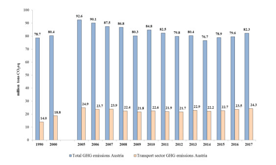
[2]
Austrian Federal Environmental Agency (2019) Austria's Annual Greenhouse Gas Inventory 1990-2017. Report REP-0672. Vienna: Umweltbundesamt.
[3]
Baumol W (1972) On taxation and the Control of Externalities. Amer Econ Rev 62: 307-321.
[4]
Baumol W, Oates W (1971) The Use of Standards and Pricing for the Protection of the Environment. Swedish J Econ 73: 42-54. doi: 10.2307/3439132
[5]
Bointner R, Biermayr P, Goers S, et al. (2013) Wirtschaftskraft Erneuerbarer Energie in Österreich und Erneuerbare Energie in Zahlen. Blue Globe Report #1/2013. Vienna: Austrian Climate and Energy Fund.
[6]
Breuss F, Steininger K (1995) Reducing the Greenhouse Effect in Austria. A General Equilibrium Evaluation of CO2-Policy-Options. EI Working Papers, Vienna.
[7]
Brons M, Nijkamp P, Pels E, et al. (2008) A meta-analysis of the price elasticity of gasoline demand. A SUR approach. Energ Econ 30: 2105-2122. doi: 10.1016/j.eneco.2007.08.004
[8]
Druckman A, Jackson T (2009) The carbon footprint of UK households 1990-2004: a socio-economically disaggregated, quasi-multi-regional input-output model. Ecol Econ 68: 2066-2077. doi: 10.1016/j.ecolecon.2009.01.013
[9]
European Environment Agency (2018) Transport greenhouse gas emissions. Available from: https://www.eea.europa.eu/airs/2018/resource-efficiency-and-low-carbon-economy/transport-ghg-emissions
[10]
Federal Ministry of Austria for Sustainability and Tourism and Federal Ministry of Austria for Transport, Innovation and Technology (2018) #mission2030. Austrian Climate and Energy Strategy. Vienna: Federal Ministry of Austria for Sustainability and Tourism and Federal Ministry of Austria for Transport, Innovation and Technology.
[11]
Goers S, Baresch M, Tichler R, et al. (2015) MOVE2-Simulation model of the (Upper) Austrian economy with a special focus on energy including the socio-economic module MOVE2social-integration of income, age and gender. Linz: Energieinstitut at the Johannes Kepler University.
[12]
Goers S, Schneider F (2019) Austria's Path to a Climate-Friendly Society and Economy-Contributions of an Environmental Tax Reform. Modern Economy 10: 1369-1384. doi: 10.4236/me.2019.105092
[13]
Goulder L (1995) Environmental taxation and the double dividend: A reader's guide. Int Tax Public Finan 2: 157-183. doi: 10.1007/BF00877495
[14]
Goulder L, Parry I, Burtraw D (1997) Revenue-Raising versus Other Approaches to Environmental Protection: The Critical Significance of Preexisting Tax Distortions. Rand J Econ 28: 708-731. doi: 10.2307/2555783
[15]
Hymel KM, Small KA, Van Dender K (2010) Induced demand and rebound effects in road transport. Transport Res B 44: 1220-1241. doi: 10.1016/j.trb.2010.02.007
[16]
Kirchner M, Sommer M, Kratena K, et al. (2019) CO2 Taxes, Equity and the Double Dividend: Macroeconomic Model Simulations for Austria. Energ Policy 126: 295-314. doi: 10.1016/j.enpol.2018.11.030
[17]
Köppl A, Kettner C, Kletzan-Slamanig D, et al. (2014) Energy Transition in Austria: Designing Mitigation Wedges. Energy Environ 25: 281-304.
[18]
Moser S, Mayrhofer J, Schmidt R, et al. (2018) Socioeconomic cost-benefit-analysis of seasonal heat storages in district heating systems with industrial waste heat integration. Energy 160: 868-874. doi: 10.1016/j.energy.2018.07.057
[19]
Ottelin J, Heinonen J, Junnila S (2018) Carbon and material footprints of a welfare state: Why and how governments should enhance green investments. Environ Sci Policy 86: 1-10. doi: 10.1016/j.envsci.2018.04.011
[20]
Pearce D (1991) The Role of Carbon Taxes in Adjusting to Global Warming. Econ J 101: 938-948. doi: 10.2307/2233865
[21]
Shammin M, Bullard C (2009) Impact of cap-and-trade policies for reducing greenhouse gas emissions on US households. Ecol Econ 68: 2432-2438. doi: 10.1016/j.ecolecon.2009.03.024
[22]
Sims R, Schaeffer R, Creutzig F, et al. (2014) Transport, In: Edenhofer O, Pichs-Madruga R, Sokona Y, Climate Change 2014: Mitigation of Climate Change. Contribution of Working Group III to the Fifth Assessment Report of the Intergovernmental Panel on Climate Change, Cambridge, New York: Cambridge University Press.
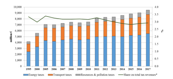
[23]
Statistik Austria (2019a) Ökosteuern. Available from: http://statistik.gv.at/web_de/statistiken/energie_umwelt_innovation_mobilitaet/energie_und_umwelt/umwelt/oeko-steuern/index.html
[24]
Statistik Austria (2019b) Kraftfahrzeuge-Neuzulassungen. Available from: http://www.statistik.at/web_de/statistiken/energie_umwelt_innovation_mobilitaet/verkehr/strasse/kraftfahrzeuge_-_neuzulassungen/index.html
[25]
Steinmüller H, Tichler R, Kienberger T, et al. (2017) Smart Exergy Leoben: Exergetische Optimierung der Energieflüsse für eine smarte Industriestadt Leoben. Vienna: Austrian Climate and Energy Fund.
[26]
Tichler R (2009) Optimale Energiepreise und Auswirkungen von Energiepreisveränderungen auf die oberösterreichische Volkswirtschaft. Analyse unter Verwendung des neu entwickelten Simulationsmodells MOVE. Linz: Energiewissenschaftliche Studien.
[27]
Titelbach G, Leitner G, van Linthoudt J-M (2018) Verteilungswirkungen potentieller Verkehrsmaßnahmen in Österreich. Research Report. Vienna: Institute for Advanced Studies.
[28]
Yeo S (2019) Where climate cash is flowing and why it's not enough. Nature 573: 328-331. doi: 10.1038/d41586-019-02712-3
This article has been cited by:
1.
Moiz Tariq, Azam Khan, Asad Ullah, Bakht Zamin, Kazem Reza Kashyzadeh, Mahmood Ahmad,
Gene Expression Programming for Estimating Shear Strength of RC Squat Wall,
2022,
12,
2075-5309,
918,
10.3390/buildings12070918
2.
Mubashar Arshad, Azad Hussain, Ashraf Elfasakhany, Soumaya Gouadria, Jan Awrejcewicz, Witold Pawłowski, Mohamed Abdelghany Elkotb, Fahad M. Alharbi,
Magneto-Hydrodynamic Flow above Exponentially Stretchable Surface with Chemical Reaction,
2022,
14,
2073-8994,
1688,
10.3390/sym14081688
3.
Mubashar Arshad, Azad Hussain, Ali Hassan, Ilyas Khan, Mohamed Badran, Sadok Mehrez, Ashraf Elfasakhany, Thabet Abdeljawad, Ahmed M. Galal,
Heat Transfer Analysis of Nanostructured Material Flow over an Exponentially Stretching Surface: A Comparative Study,
2022,
12,
2079-4991,
1204,
10.3390/nano12071204
4.
O. Yu. Kosukha, Iu. M. Shevchuk,
A SYSTEM OF INTELLECTUAL ANALYSIS AND PREDICTION OF REACTIONS TO NEWS BASED ON DATA FROM TELEGRAM CHANNELS,
2022,
27069680,
59,
10.17721/2706-9699.2022.2.07
5.
Mubashar Arshad, Hanen Karamti, Jan Awrejcewicz, Dariusz Grzelczyk, Ahmed M. Galal,
Thermal Transmission Comparison of Nanofluids over Stretching Surface under the Influence of Magnetic Field,
2022,
13,
2072-666X,
1296,
10.3390/mi13081296
6.
Kazem Reza Kashyzadeh, Nima Amiri, Siamak Ghorbani, Kambiz Souri,
Prediction of Concrete Compressive Strength Using a Back-Propagation Neural Network Optimized by a Genetic Algorithm and Response Surface Analysis Considering the Appearance of Aggregates and Curing Conditions,
2022,
12,
2075-5309,
438,
10.3390/buildings12040438
7.
Peter Kolapo, Gafar Omotayo Oniyide, Khadija Omar Said, Abiodun Ismail Lawal, Moshood Onifade, Prosper Munemo,
An Overview of Slope Failure in Mining Operations,
2022,
2,
2673-6489,
350,
10.3390/mining2020019
8.
O. G. Nakonechnyi, O. A. Kapustian, Iu. M. Shevchuk, M. V. Loseva, O. Yu. Kosukha,
A intellectual system of analysis of reactions to news based on data from Telegram channels,
2022,
18125409,
55,
10.17721/1812-5409.2022/3.7
9.
Feezan Ahmad, Xiaowei Tang, Jilei Hu, Mahmood Ahmad, Behrouz Gordan,
Improved Prediction of Slope Stability under Static and Dynamic Conditions Using Tree-Based Models,
2023,
137,
1526-1506,
455,
10.32604/cmes.2023.025993
10.
Gamil M. S. Abdullah, Mahmood Ahmad, Muhammad Babur, Muhammad Usman Badshah, Ramez A. Al-Mansob, Yaser Gamil, Muhammad Fawad,
Boosting-based ensemble machine learning models for predicting unconfined compressive strength of geopolymer stabilized clayey soil,
2024,
14,
2045-2322,
10.1038/s41598-024-52825-7
11.
Congcong Zhou, Zhenzhong Shen, Liqun Xu, Yiqing Sun, Wenbing Zhang, Hongwei Zhang, Jiayi Peng,
Global Sensitivity Analysis Method for Embankment Dam Slope Stability Considering Seepage–Stress Coupling under Changing Reservoir Water Levels,
2023,
11,
2227-7390,
2836,
10.3390/math11132836
12.
Mojtaba Yari, Saeed Jamali, Gamil M. S. Abdullah, Mahmood Ahmad, Muhammad Usman Badshah, Taoufik Najeh,
Development a risk assessment method for dimensional stone quarries,
2024,
14,
2045-2322,
10.1038/s41598-024-64276-1
13.
Prashanth Ragam, N. Kushal Kumar, Jubilson E. Ajith, Guntha Karthik, Vivek Kumar Himanshu, Divya Sree Machupalli, Bhatawdekar Ramesh Murlidhar,
Estimation of slope stability using ensemble-based hybrid machine learning approaches,
2024,
11,
2296-8016,
10.3389/fmats.2024.1330609
14.
Mohammad A. Al‑Zubi, Mahmood Ahmad, Shahriar Abdullah, Beenish Jehan Khan, Wajeeha Qamar, Gamil M. S. Abdullah, Roberto Alonso González-Lezcano, Sonjoy Paul, N. S. Abd EL-Gawaad, Tariq Ouahbi, Muhammad Kashif,
Long short term memory networks for predicting resilient Modulus of stabilized base material subject to wet-dry cycles,
2024,
14,
2045-2322,
10.1038/s41598-024-79588-5
15.
Mohammad Sadegh Barkhordari, Mohammad Mahdi Barkhordari, Danial Jahed Armaghani, Edy Tonnizam Mohamad, Behrouz Gordan,
GUI-based platform for slope stability prediction under seismic conditions using machine learning algorithms,
2024,
4,
2730-9886,
145,
10.1007/s44150-024-00112-4
16.
Gongfa Chen, Wei Deng, Mansheng Lin, Jianbin Lv,
Slope stability analysis based on convolutional neural network and digital twin,
2023,
118,
0921-030X,
1427,
10.1007/s11069-023-06055-1
17.
Na Lu, Bin Meng,
Risk Analysis of Airplane Upsets in Flight: An Integrated System Framework and Analysis Methodology,
2023,
10,
2226-4310,
446,
10.3390/aerospace10050446
18.
Bamaiyi Usman Aliyu, Linrong Xu, Al-Amin Danladi Bello, Abdulrahman Shuaibu, Robert M. Kalin, Abdulaziz Ahmad, Nahidul Islam, Basit Raza,
Prediction of Railway Embankment Slope Hydromechanical Properties under Bidirectional Water Level Fluctuations,
2024,
14,
2076-3417,
3402,
10.3390/app14083402
19.
Arsalan Mahmoodzadeh, Abed Alanazi, Adil Hussein Mohammed, Ahmed Babeker Elhag, Abdullah Alqahtani, Shtwai Alsubai,
An optimized model based on the gene expression programming method to estimate safety factor of rock slopes,
2024,
120,
0921-030X,
1665,
10.1007/s11069-023-06152-1
Sebastian Goers, Friedrich Schneider. Economic, ecological and social benefits through redistributing revenues from increased mineral oil taxation in Austria: A triple dividend[J]. Green Finance, 2019, 1(4): 442-456. doi: 10.3934/GF.2019.4.442
*Note 0: Unstable; 1: Stable; (*) represents the test dataset.
Figure 1. Total and transport sector GHG emissions in Austria
Figure 2. Environmental tax revenues in Austria. Note: *Total revenues from taxes and social contributions after deduction of amounts assessed but unlikely to be collected