Role of PTH in the Renal Handling of Phosphate

Rebecca D. Murray; Eleanor D. Lederer; Syed J. Khundmiri; Rebecca D. Murray; Eleanor D. Lederer; Syed J. Khundmiri

doi:10.3934/medsci.2015.3.162

AIMS Medical Science

2015, Volume 2, Issue 3: 162-181. doi: 10.3934/medsci.2015.3.162

Previous Article Next Article

Review Special Issues

Role of PTH in the Renal Handling of Phosphate

1.
Department of Physiology & Biophysics, University of Louisville, Louisville, KY, USA;
2.
Department of Medicine, University of Louisville, Louisville, KY, USA;
3.
Robley Rex VAMC, Louisville, KY, USA;
4.
Department of Physiology and Biophysics, Howard University College of Medicine, Washington, DC, USA

Received: 26 April 2015 Accepted: 31 July 2015 Published: 10 August 2015

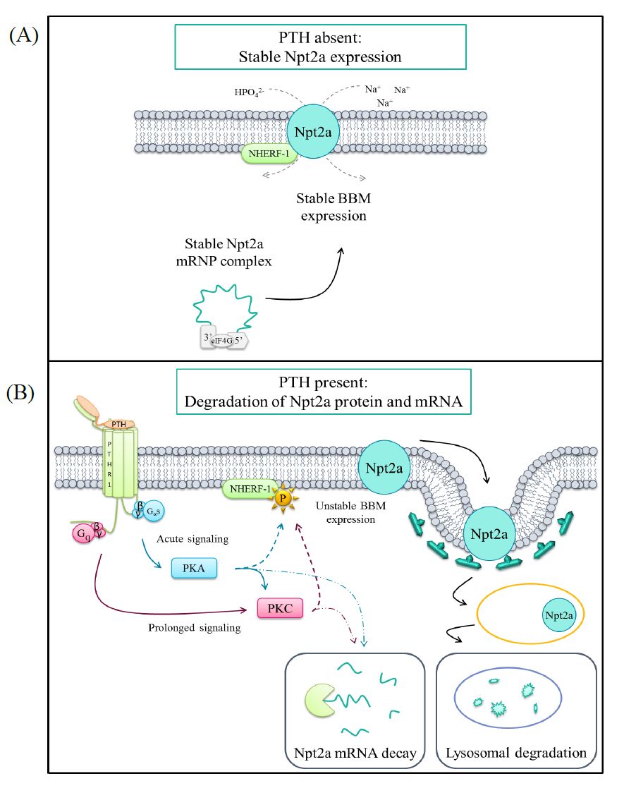
Parathyroid hormone (PTH) is one of the primary phosphaturic hormones in the body. The type IIa sodium-phosphate cotransporter (Npt2a) is expressed in the apical membrane of the renal proximal tubule and is responsible for the reabsorption of the majority of the filtered load of phosphate. PTH acutely induces phosphaturia through the rapid stimulation of endocytosis of Npt2a and its subsequent lysosomal degradation. This review focuses on the homeostatic mechanisms underlying serum phosphate, with particular focus on the regulation of the phosphate transporter Npt2a by PTH within the renal proximal tubule. Additionally, the proximal tubular PTH-stimulated signaling events as they relate to PTH-induced phosphaturia are also highlighted. Lastly, we discuss recent findings by our lab concerning novel regulatory mechanisms of PTH-mediated reductions in Npt2a expression.
- phosphate,
- PTH,
- GPCR signaling,
- renal proximal tubule,
- Npt2a
Citation: Rebecca D. Murray, Eleanor D. Lederer, Syed J. Khundmiri. Role of PTH in the Renal Handling of Phosphate[J]. AIMS Medical Science, 2015, 2(3): 162-181. doi: 10.3934/medsci.2015.3.162

Related Papers:

Abstract

Parathyroid hormone (PTH) is one of the primary phosphaturic hormones in the body. The type IIa sodium-phosphate cotransporter (Npt2a) is expressed in the apical membrane of the renal proximal tubule and is responsible for the reabsorption of the majority of the filtered load of phosphate. PTH acutely induces phosphaturia through the rapid stimulation of endocytosis of Npt2a and its subsequent lysosomal degradation. This review focuses on the homeostatic mechanisms underlying serum phosphate, with particular focus on the regulation of the phosphate transporter Npt2a by PTH within the renal proximal tubule. Additionally, the proximal tubular PTH-stimulated signaling events as they relate to PTH-induced phosphaturia are also highlighted. Lastly, we discuss recent findings by our lab concerning novel regulatory mechanisms of PTH-mediated reductions in Npt2a expression.

References

[1]	Gates F, Grant J (1927) Experimental Observations on Irradiated, Normal, and Partially Parathyroidectomized Rabbits. J Exp Med 45:125-137.
[2]	Beck L, Karaplis A, Amizuka N, et al. (1998) Targeted inactivation of Npt2 in mice leads to severe renal phosphate wasting, hypercalciuria, and skeletal abnormalities. Proc Natl Acad Sci U S A 95:5372-5377. doi: 10.1073/pnas.95.9.5372
[3]	Hedbäck G, Odén A (1998) Increased risk of death from primary hyperparathyroidism－an update. Eur J Clin Invest 28:271-276. doi: 10.1046/j.1365-2362.1998.00289.x
[4]	Raue F (1998) Increased incidence of cardiovascular diseases in primary hyperparathyroidism－a cause for more aggressive treatment? Eur J Clin Invest 28:277-278. doi: 10.1046/j.1365-2362.1998.00290.x
[5]	Conzo G, Perna A, Candela G, et al. (2012) Long-term outcomes following “presumed” total parathyroidectomy for secondary hyperparathyroidism of chronic kidney disease. G Chir 33:379-382.
[6]	Bansal V (1990) Serum Inorganic Phosphorus. In: Walker HK, Hall WD, Hurst JW (eds) Clin. Methods Hist. Phys Lab Exam 895-899.
[7]	Menon M, Ix J (2013) Dietary phosphorus, serum phosphorus, and cardiovascular disease. Ann N Y Acad Sci 1301:21-26. doi: 10.1111/nyas.12283
[8]	Baker S, Worthley L (2002) The essentials of calcium, magnesium and phosphate metabolism: part I. Physiology. Crit Care Resusc 4:301-306.
[9]	Penido M, Alon U (2012) Phosphate homeostasis and its role in bone health. Pediatr Nephrol 27:2039-2048. doi: 10.1007/s00467-012-2175-z
[10]	Mason J (2011) Vitamins, trace minerals, and other micronutrients. In: Goldman L, Ausiello D, eds. Cecil Medicine. 24th ed. Philadelphia, Pa: Saunders Elsevier; chap 225.
[11]	Takeda E, Taketani Y, Sawada N, et al. (2004) The regulation and function of phosphate in the human body. Biofactors 21:345-355. doi: 10.1002/biof.552210167
[12]	Loghman-Adham M (1997) Adaptation to changes in dietary phosphorus intake in health and in renal failure. J Lab Clin Med 129:176-188. doi: 10.1016/S0022-2143(97)90137-2
[13]	Katai K, Miyamoto K, Kishida S, et al. (1999) Regulation of intestinal Na⁺-dependent phosphate co-transporters by a low-phosphate diet and 1,25-dihydroxyvitamin D3. Biochem J 343 Pt 3:705-712.
[14]	Hildmann B, Storelli C, Danisi G, et al. (1982) Regulation of Na⁺-Pi cotransport by 1,25-dihydroxyvitamin D3 in rabbit duodenal brush-border membrane. Am J Physiol 242:G533-G539.
[15]	Danisi G, Caverzasio J, Trechsel U, et al. (1990) Phosphate transport adaptation in rat jejunum and plasma level of 1,25-dihydroxyvitamin D3. Scand J Gastroenterol 25:210-215.
[16]	Kido S, Kaneko I, Tatsumi S, et al. (2013) Vitamin D and type II sodium-dependent phosphate cotransporters. Contrib Nephrol 180:86-97. doi: 10.1159/000346786
[17]	Kaneko I, Segawa H, Furutani J, et al. (2011) Hypophosphatemia in vitamin D receptor null mice: Effect of rescue diet on the developmental changes in renal Na⁺-dependent phosphate cotransporters. Pflugers Arch Eur J Physiol 461:77-90. doi: 10.1007/s00424-010-0888-z
[18]	Ikeda K, Takeshita S (2014) Factors and mechanisms involved in the coupling from bone resorption to formation: how osteoclasts talk to osteoblasts. J bone Metab 21:163-167. doi: 10.11005/jbm.2014.21.3.163
[19]	Agus Z, Puscttrr J, Senesky D, et al. (1971) Mode of Action of Parathyroid Hormone and cyclic adenosine 3',5'-monophosphate on Renal Tubular Phosphate Reabsorption in the Dog. J Clin Invest 50:617-626. doi: 10.1172/JCI106532
[20]	Collins J, Bai L, Ghishan F (2004) The SLC20 family of proteins: dual functions as sodium-phosphate cotransporters and viral receptors. Pflugers Arch 447:647-652. doi: 10.1007/s00424-003-1088-x
[21]	Nishimura M, Naito S (2008) Tissue-specific mRNA Expression Profiles of Human Solute Carrier Transporter Superfamilies. Drug Metab Pharmacokinet 23:22-44. doi: 10.2133/dmpk.23.22
[22]	Villa-Bellosta R, Ravera S, Sorribas V, et al. (2009) The Na⁺-Pi cotransporter PiT-2 (SLC20A2) is expressed in the apical membrane of rat renal proximal tubules and regulated by dietary Pi. Am J Physiol Renal Physiol 296:F691-699. doi: 10.1152/ajprenal.90623.2008
[23]	Bacconi A, Virkki L V, Biber J, et al. (2005) Renouncing electroneutrality is not free of charge: switching on electrogenicity in a Na+-coupled phosphate cotransporter. Proc Natl Acad Sci U S A 102:12606-12611. doi: 10.1073/pnas.0505882102
[24]	Renkema K, Alexander R, Bindels R, et al. (2008) Calcium and phosphate homeostasis: concerted interplay of new regulators. Ann Med 40:82-91. doi: 10.1080/07853890701689645
[25]	Tenenhouse H (2007) Phosphate transport: molecular basis, regulation and pathophysiology. J Steroid Biochem Mol Biol 103:572-577. doi: 10.1016/j.jsbmb.2006.12.090
[26]	Forster IC, Hernando N, Biber J, et al. (2006) Proximal tubular handling of phosphate: A molecular perspective. Kidney Int 70:1548-1559. doi: 10.1038/sj.ki.5001813
[27]	Custer M, Lötscher M, Biber J, et al. (1994) Expression of Na-P(i) cotransport in rat kidney: localization by RT-PCR and immunohistochemistry. Am J Physiol 266:F767-F774.
[28]	Picard N, Capuano P, Stange G, et al. (2010) Acute parathyroid hormone differentially regulates renal brush border membrane phosphate cotransporters. Pflugers Arch Eur J Physiol 460:677-687. doi: 10.1007/s00424-010-0841-1
[29]	Segawa H, Kaneko I, Takahashi A, et al. (2002) Growth-related renal type II Na/Pi cotransporter. J Biol Chem 277:19665-19672. doi: 10.1074/jbc.M200943200
[30]	Chau H, El-Maadawy S, McKee M, et al. (2003) Renal calcification in mice homozygous for the disrupted type IIa Na/Pi cotransporter gene Npt2. J Bone Miner Res 18:644-657. doi: 10.1359/jbmr.2003.18.4.644
[31]	Levi M, Lötscher M, Sorribas V, et al. (1994) Cellular mechanisms of acute and chronic adaptation of rat renal P(i) transporter to alterations in dietary P(i). Am J Physiol 267:F900-908.
[32]	Pfister M, Hilfiker H, Forgo J, et al. (1998) Cellular mechanisms involved in the acute adaptation of OK cell Na/Pi-cotransport to high- or low-Pi medium. Pflugers Arch 435:713-719. doi: 10.1007/s004240050573
[33]	Tenenhouse H (2005) Regulation of phosphorus homeostasis by the type iia na/phosphate cotransporter. Annu Rev Nutr 25:197-214. doi: 10.1146/annurev.nutr.25.050304.092642
[34]	Murer H, Hernando N, Forster I, et al. (2000) Proximal tubular phosphate reabsorption: molecular mechanisms. Physiol Rev 80:1373-1409.
[35]	Khan S, Canales B (2011) Ultrastructural investigation of crystal deposits in Npt2a knockout mice: are they similar to human Randall's plaques? J Urol 186:1107-1113. doi: 10.1016/j.juro.2011.04.109
[36]	Iwaki T, Sandoval-Cooper M, Tenenhouse H, et al. (2008) A missense mutation in the sodium phosphate co-transporter Slc34a1 impairs phosphate homeostasis. J Am Soc Nephrol 19:1753-1762. doi: 10.1681/ASN.2007121360
[37]	Myakala K, Motta S, Murer H, et al. (2014) Renal-specific and inducible depletion of NaPi-IIc/Slc34a3, the cotransporter mutated in HHRH, does not affect phosphate or calcium homeostasis in mice. Am J Physiol - Ren Physiol 306:F833-F843. doi: 10.1152/ajprenal.00133.2013
[38]	Segawa H, Onitsuka A, Kuwahata M, et al (2009) Type IIc sodium-dependent phosphate transporter regulates calcium metabolism. J Am Soc Nephrol 20:104-113. doi: 10.1681/ASN.2008020177
[39]	Haussler M, Whitfield G, Kaneko I, et al. (2012) The role of vitamin D in the FGF23, klotho, and phosphate bone-kidney endocrine axis. Rev Endocr Metab Disord 13:57-69. doi: 10.1007/s11154-011-9199-8
[40]	Stechman M, Loh N, Thakker R (2009) Genetic causes of hypercalciuric nephrolithiasis. Pediatr Nephrol 24:2321-32. doi: 10.1007/s00467-008-0807-0
[41]	Prié D, Beck L, Friedlander G, et al. (2004) Sodium-phosphate cotransporters, nephrolithiasis and bone demineralization. Curr Opin Nephrol Hypertens 13:675-681. doi: 10.1097/00041552-200411000-00015
[42]	Magen D, Berger L, Coady M, et al. (2010) A Loss-of-Function Mutation in NaPi-IIa and Renal Fanconi's Syndrome. N Engl J Med 362:1102-1109. doi: 10.1056/NEJMoa0905647
[43]	Rajagopal A, Débora B, James T, et al. (2014) Exome sequencing identifies a novel homozygous mutation in the phosphate transporter SLC34A1 in hypophosphatemia and nephrocalcinosis. J Clin Endocrinol Metab jc20141517.
[44]	Kenny J, Lees M, Drury S, et al. (2011) Sotos syndrome, infantile hypercalcemia, and nephrocalcinosis: a contiguous gene syndrome. Pediatr Nephrol 26:1331-1334. doi: 10.1007/s00467-011-1884-z
[45]	Schlingmann K, Ruminska J, Kaufmann M, et al. (2015) Autosomal-Recessive Mutations in SLC34A1 Encoding Sodium-Phosphate Cotransporter 2A Cause Idiopathic Infantile Hypercalcemia. J Am Soc Nephrol 1-11.
[46]	Kestenbaum B, Glazer N, Köttgen A, et al. (2010) Common genetic variants associate with serum phosphorus concentration. J Am Soc Nephrol 21:1223-1232. doi: 10.1681/ASN.2009111104
[47]	Silver J, Naveh-Many T (2009) Phosphate and the parathyroid. Kidney Int 75:898-905. doi: 10.1038/ki.2008.642
[48]	Bergwitz C, Jüppner H (2010) Regulation of phosphate homeostasis by PTH, vitamin D, and FGF23. Annu Rev Med 61:91-104. doi: 10.1146/annurev.med.051308.111339
[49]	Caniggia A, Lore F, di Cairano G, et al. (1987) Main endocrine modulators of vitamin D hydroxylases in human pathophysiology. J Steroid Biochem 27:815-824. doi: 10.1016/0022-4731(87)90154-3
[50]	Wang W, Li C, Kwon T, et al. (2004) Reduced expression of renal Na⁺ transporters in rats with PTH-induced hypercalcemia. Am J Physiol Ren Physiol 286:534-545. doi: 10.1152/ajprenal.00044.2003
[51]	Haramati A, Knox F (1983) Tubular capacity of phosphate transport in phosphate-deprived rats: effects of nicotinamide and PTH. Am J Physiol 244:F178-F184.
[52]	Guo J, Song L, Liu M, et al. (2013) Activation of a non-cAMP/PKA signaling pathway downstream of the PTH/PTHrP receptor is essential for a sustained hypophosphatemic response to PTH infusion in male mice. Endocrinology 154:1680-1689. doi: 10.1210/en.2012-2240
[53]	Yamamoto H, Tani Y, Kobayashi K, et al. (2005) Alternative promoters and renal cell-specific regulation of the mouse type IIa sodium-dependent phosphate cotransporter gene. Biochim Biophys Acta 1732:43-52. doi: 10.1016/j.bbaexp.2005.11.003
[54]	Silver J, Russell J, Sherwood L (1985) Regulation by vitamin D metabolites of messenger ribonucleic acid for preproparathyroid hormone in isolated bovine parathyroid cells. Proc Natl Acad Sci U S A 82:4270-4273. doi: 10.1073/pnas.82.12.4270
[55]	Silver J, Yalcindag C, Sela-Brown A, et al. (1999) Regulation of the parathyroid hormone gene by vitamin D, calcium and phosphate. Kidney Int 73:S2-7.
[56]	Barthel T, Mathern D, Whitfield G, et al. (2007) 1,25-Dihydroxyvitamin D3/VDR-mediated induction of FGF23 as well as transcriptional control of other bone anabolic and catabolic genes that orchestrate the regulation of phosphate and calcium mineral metabolism. J Steroid Biochem Mol Biol 103:381-388. doi: 10.1016/j.jsbmb.2006.12.054
[57]	Friedlaender M, Wald H, Dranitzki-Elhalel M, et al. (2001) Vitamin D reduces renal NaPi-2 in PTH-infused rats: complexity of vitamin D action on renal Pi handling. Am J Physiol Ren Physiol 281:428-433.
[58]	Weinman E, Steplock D, Wang Y, et al. (1995) Characterization of a Protein Cofactor that Mediates Protein Kinase A Regulation of the Renal Brush Border Membrane Na⁺-H⁺ Exchanger. J Clin Invest 95:2143-2149. doi: 10.1172/JCI117903
[59]	Weinman E, Lederer E (2012) NHERF-1 and the regulation of renal phosphate reabsoption: a tale of three hormones. Am J Physiol Renal Physiol 303:F321-327. doi: 10.1152/ajprenal.00093.2012
[60]	Weinman E, Biswas R, Peng G, et al. (2007) Parathyroid hormone inhibits renal phosphate transport by phosphorylation of serine 77 of sodium-hydrogen exchanger regulatory factor-1. J Clin Invest 117:3412-3420. doi: 10.1172/JCI32738
[61]	Mahon M, Segre G (2004) Stimulation by parathyroid hormone of a NHERF-1-assembled complex consisting of the parathyroid hormone I receptor, phospholipase Cbeta, and actin increases intracellular calcium in opossum kidney cells. J Biol Chem 279:23550-23558. doi: 10.1074/jbc.M313229200
[62]	Khundmiri S, Rane M, Lederer E (2003) Parathyroid hormone regulation of type II sodium-phosphate cotransporters is dependent on an A kinase anchoring protein. J Biol Chem 278:10134-10141. doi: 10.1074/jbc.M211775200
[63]	Lederer E, Khundmiri S, Weinman E (2003) Role of NHERF-1 in regulation of the activity of Na-K ATPase and sodium-phosphate co-transport in epithelial cells. J Am Soc Nephrol 14:1711-1719. doi: 10.1097/01.ASN.0000072744.67971.21
[64]	Hernando N, Deliot N, Gisler S, et al. (2002) PDZ-domain interactions and apical expression of type IIa Na/Pi cotransporters. Proc Natl Acad Sci U S A 99:11957-11962. doi: 10.1073/pnas.182412699
[65]	Mahon M, Cole J, Lederer E, et al. (2003) Na⁺/H⁺ exchanger-regulatory factor 1 mediates inhibition of phosphate transport by parathyroid hormone and second messengers by acting at multiple sites in opossum kidney cells. Mol Endocrinol 17:2355-2364. doi: 10.1210/me.2003-0043
[66]	Weinman E, Steplock D, Shenolikar S, et al. (2011) Dynamics of PTH-induced disassembly of Npt2a/NHERF-1 complexes in living OK cells. Am J Physiol Renal Physiol 300:F231-F235. doi: 10.1152/ajprenal.00532.2010
[67]	Kempson S, Lötscher M, Kaissling B, et al. (1995) Parathyroid hormone action on phosphate transporter mRNA and protein in rat renal proximal tubules. Am J Physiol 268:F784-791.
[68]	Pfister M, Ruf I, Stange G, et al. (1998) Parathyroid hormone leads to the lysosomal degradation of the renal type II Na/Pi cotransporter. Proc Natl Acad Sci U S A 95:1909-1914. doi: 10.1073/pnas.95.4.1909
[69]	Pfister M, Lederer E, Forgo J, et al. (1997) Parathyroid Hormone-dependent Degradation of Type II Na⁺/Pi Cotransporters. J Biol Chem 272:20125-20130. doi: 10.1074/jbc.272.32.20125
[70]	Abou-Samra A, Jüppner H, Force T, et al. (1992) Expression cloning of a common receptor for parathyroid hormone and parathyroid hormone-related peptide from rat osteoblast-like cells: a single receptor stimulates intracellular accumulation of both cAMP and inositol trisphosphates and increases intracel. Proc Natl Acad Sci U S A 89:2732-2736. doi: 10.1073/pnas.89.7.2732
[71]	Watson P, Fraher L, Hendy G, et al. (2000) Nuclear localization of the type 1 PTH/PTHrP receptor in rat tissues. J Bone Miner Res 15:1033-1044. doi: 10.1359/jbmr.2000.15.6.1033
[72]	Friedman P, Gesek F, Morley P, et al. (1999) Cell-specific signaling and structure-activity relations of parathyroid hormone analogs in mouse kidney cells. Endocrinology 140:301-309.
[73]	Amizuka N, Lee H, Kwan M, et al. (1997) Cell-Specific Expression of the Parathyroid Hormone (PTH)/PTH-Related Peptide Receptor Gene in Kidney from Kidney-Specific and Ubiquitous Promoters. Endocrinology 138:469-481.
[74]	Taylor C, Tovey S (2012) From parathyroid hormone to cytosolic Ca²⁺ signals. Biochem Soc Trans 40:147-52. doi: 10.1042/BST20110615
[75]	Muff R, Fischer J, Biber J, et al. (1992) Parathyroid Hormone Receptors in Control of Proximal Tubule Function. Annu Rev Physiol 54:67-79. doi: 10.1146/annurev.ph.54.030192.000435
[76]	Suarez F, Silve C (1992) Effect of Parathyroid Hormone on Arachidonic Acid Metabolism in Mouse Osteoblasts: Permissive Action of Dexamethasone. Endocrinology 130:592-598.
[77]	Cole J (1999) Parathyroid hormone activates mitogen-activated protein kinase in opossum kidney cells. Endocrinology 140:5771-5779. doi: 10.1210/endo.140.12.7173
[78]	Khundmiri S, Ameen M, Delamere N, et al. (2008) PTH-mediated regulation of Na⁽⁺⁾-K⁽⁺⁾-ATPase requires Src kinase-dependent ERK phosphorylation. Am J Physiol - Ren Physiol 295:F426-F437. doi: 10.1152/ajprenal.00516.2007
[79]	Bacic D, Schulz N, Biber J, et al. (2003) Involvement of the MAPK-kinase pathway in the PTH-mediated regulation of the proximal tubule type IIa Na⁺/Pi cotransporter in mouse kidney. Pflugers Arch 446:52-60.
[80]	Yang S, Xiao L, Li J, et al. (2013) Role of guanine-nucleotide exchange factor Epac in renal physiology and pathophysiology. Am J Physiol Ren Physiol 304:F831-839. doi: 10.1152/ajprenal.00711.2012
[81]	Li Y, Konings I, Zhao J, et al. (2008) Renal expression of exchange protein directly activated by cAMP (Epac) 1 and 2. Am J Physiol Ren Physiol 295:F525-533. doi: 10.1152/ajprenal.00448.2007
[82]	Ostrom R, Bogard A, Gros R, et al. (2012) Choreographing the adenylyl cyclase signalosome: sorting out the partners and the steps. Naunyn Schmiedebergs Arch Pharmacol 385:5-12. doi: 10.1007/s00210-011-0696-9
[83]	Bek M, Zheng S, Xu J, et al. (2001) Differential expression of adenylyl cyclases in the rat nephron. Kidney Int 60:890-899. doi: 10.1046/j.1523-1755.2001.060003890.x
[84]	Murtazina R, Kovbasnjuk O, Zachos NC, et al. (2007) Tissue-specific regulation of sodium/proton exchanger isoform 3 activity in Na⁽⁺⁾/H⁽⁺⁾ exchanger regulatory factor 1 (NHERF1) null mice. J Biol Chem 282:25141-25151. doi: 10.1074/jbc.M701910200
[85]	Courbebaisse M, Leroy C, Bakouh N, et al. (2012) A new human NHERF1 mutation decreases renal phosphate transporter NPT2a expression by a PTH-independent mechanism. PLoS One 7:e34764. doi: 10.1371/journal.pone.0034764
[86]	Ferrandon S, Feinstein T, Castro M, et al. (2009) Sustained cyclic AMP production by parathyroid hormone receptor endocytosis. Nat Chem Biol 5:734-742. doi: 10.1038/nchembio.206
[87]	Ahlström M, Lamberg‐Allardt C (1997) Rapid Protein Kinase A—Mediated Activation of Cyclic AMP-Phosphodiesterase by Parathyroid Hormone in UMR-106 Osteoblast-like Cells. J Bone Miner Res 12:172-178. doi: 10.1359/jbmr.1997.12.2.172
[88]	Whitfield J, Isaacs R, Chakravarthy B, et al. (2001) Stimulation of protein kinase C activity in cells expressing human parathyroid hormone receptors by C- and N-terminally truncated fragments of parathyroid hormone 1-34. J Bone Miner Res 16:441-447. doi: 10.1359/jbmr.2001.16.3.441
[89]	Mahon M, Donowitz M, Yun C, et al. (2002) Na⁺/H⁺ exchanger regulatory factor 2 directs parathyroid hormone 1 receptor signalling. Nature 417:858-861. doi: 10.1038/nature00816
[90]	Jouishomme H, Whitfield J, Gagnon L, et al. (1994) Further definition of the protein kinase C activation domain of the parathyroid hormone. J Bone Miner Res 9:943-949.
[91]	Whitfield J, Isaacs R, Chakravarthy B, et al. (2001) Protein Kinase C Activity in Cells Expressing Human Parathyroid Hormone Receptors by C‐and N‐Terminally Truncated Fragments of Parathyroid Hormone 1. J Bone Miner Res 16:441-447. doi: 10.1359/jbmr.2001.16.3.441
[92]	Wang B, Yang Y, Abou-Samra A, et al. (2009) NHERF1 regulates parathyroid hormone receptor desensitization: interference with beta-arrestin binding. Mol Pharmacol 75:1189-1197. doi: 10.1124/mol.108.054486
[93]	Alonso V, Magyar C, Wang B, et al. (2011) Ubiquitination-deubiquitination balance dictates ligand-stimulated PTHR sorting. J bone Miner Res 26:2923-2934. doi: 10.1002/jbmr.494
[94]	Chauvin S, Bencsik M, Bambino T, et al. (2002) Parathyroid hormone receptor recycling: role of receptor dephosphorylation and beta-arrestin. Mol Endocrinol 16:2720-2732. doi: 10.1210/me.2002-0049
[95]	Wang B, Bisello A, Yang Y, et al. (2007) NHERF1 regulates parathyroid hormone receptor membrane retention without affecting recycling. J Biol Chem 282:36214-36222. doi: 10.1074/jbc.M707263200
[96]	Khundmiri S, Weinman E, Steplock D, et al. (2005) Parathyroid hormone regulation of NA⁺,K⁺-ATPase requires the PDZ 1 domain of sodium hydrogen exchanger regulatory factor-1 in opossum kidney cells. J Am Soc Nephrol 16:2598-2607. doi: 10.1681/ASN.2004121049
[97]	Salyer S, Lesousky N, Weinman E, et al. (2011) Dopamine regulation of Na⁺-K⁺-ATPase requires the PDZ-2 domain of sodium hydrogen regulatory factor-1 (NHERF-1) in opossum kidney cells. Am J Physiol Cell Physiol 300:C425-C434. doi: 10.1152/ajpcell.00357.2010
[98]	Tawfeek H, Abou-Samra A (2004) Important role for the V-type H⁺-ATPase and the Golgi apparatus in the recycling of PTH/PTHrP receptor. Am J Physiol Endocrinol Metab 286:704-710.
[99]	Pickard B, Hodsman A, Fraher L, et al. (2007) Type 1 parathyroid hormone receptor (PTH1R) nuclear trafficking: regulation of PTH1R nuclear-cytoplasmic shuttling by importin-alpha/beta and chromosomal region maintenance 1/exportin 1. Endocrinology 148:2282-2289. doi: 10.1210/en.2007-0157
[100]	Silverstein D, Spitzer A, Barac-Nieto M (2005) Parathormone sensitivity and responses to protein kinases in subclones of opossum kidney cells. Pediatr Nephrol 20:721-724. doi: 10.1007/s00467-005-1832-x
[101]	Nagai S, Okazaki M, Segawa H, et al. (2011) Acute down-regulation of sodium-dependent phosphate transporter NPT2a involves predominantly the cAMP/PKA pathway as revealed by signaling-selective parathyroid hormone analogs. J Biol Chem 286:1618-1626. doi: 10.1074/jbc.M110.198416
[102]	Cole J, Eber S, Poelling R, et al. (1987) A dual mechanism for regulation of kidney phosphate transport by parathyroid hormone. Am J Physiol 253:E221-227.
[103]	Cole J, Forte L, Eber S, et al. (1988) Regulation of sodium-dependent phosphate transport by parathyroid hormone in opossum kidney cells: Adenosine 3',5'-monophosphate-dependent and -independent mechanisms. Endocrinology 122:2981-2989. doi: 10.1210/endo-122-6-2981
[104]	Fenton R, Murray F, Dominguez J, et al. (2014) Renal phosphate wasting in the absence of adenylyl cyclase 6. J Am Soc Nephrol 1-13.
[105]	Weinstein L, Yu S, Warner D, et al. (2001) Endocrine manifestations of stimulatory G protein alpha-subunit mutations and the role of genomic imprinting. Endocr Rev 22:675-705.
[106]	Mantovani G (2011) Clinical review: Pseudohypoparathyroidism: diagnosis and treatment. J Clin Endocrinol Metab 96:3020-3030. doi: 10.1210/jc.2011-1048
[107]	Carpenter T, McPhee M, Bort R, et al. (1992) Dissociation of phosphaturia and 25(OH)D-1a-hydroxylase trophism using a novel analogue of parathyroid hormone. Am J Physiol 25:483-487.
[108]	Cunningham R, Biswas R, Brazie M, et al. (2009) Signaling pathways utilized by PTH and dopamine to inhibit phosphate transport in mouse renal proximal tubule cells. Am J Physiol Renal Physiol 296:F355-361.
[109]	Ranch D, Zhang M, Portale A, et al. (2011) Fibroblast growth factor 23 regulates renal 1,25-dihydroxyvitamin D and phosphate metabolism via the MAP kinase signaling pathway in Hyp mice. J Bone Miner Res 26:1883-1890. doi: 10.1002/jbmr.401
[110]	Kilav R, Silver J, Biber J, et al. (1995) Coordinate regulation of rat renal parathyroid hormone receptor mRNA and Na-Pi cotransporter mRNA and protein. Am J Physiol 268:F1017-1022.
[111]	Moe S, Radcliffe J, White K, et al. (2011) The pathophysiology of early-stage chronic kidney disease-mineral bone disorder (CKD-MBD) and response to phosphate binders in the rat. J Bone Miner Res 26:2672-2681. doi: 10.1002/jbmr.485
[112]	Hilfiker H, Hartmann C, Stange G, et al. (1998) Characterization of the 5 J-flanking region of OK cell type II Na-Pi cotransporter gene. 12:197-204.
[113]	Murray R, Holthouser K, Clark B, et al. (2013) Parathyroid hormone (PTH) decreases sodium-phosphate cotransporter type IIa (NpT2a) mRNA stability. Am J Physiol Renal Physiol 304:F1076-1085. doi: 10.1152/ajprenal.00632.2012
[114]	Moz Y, Silver J, Naveh-Many T. (1999) Protein-RNA Interactions Determine the Stability of the Renal NaPi-2 Cotransporter mRNA and Its Translation in Hypophosphatemic Rats. J Biol Chem 274:25266-25272. doi: 10.1074/jbc.274.36.25266
[115]	Moz Y, Silver J, Naveh-Many T. (2003) Characterization of cis-acting element in renal NaPi-2 cotransporter mRNA that determines mRNA stability. Am J Physiol Renal Physiol 284:F663-670. doi: 10.1152/ajprenal.00332.2002
[116]	Noronha-Blob L, Sacktor B. (1986) Inhibition by glucocorticoids of phosphate transport in primary cultured renal cells. J Biol Chem 261:2164-2169.

Reader Comments

Your name:*

Email:*
© 2015 the Author(s), licensee AIMS Press. This is an open access article distributed under the terms of the Creative Commons Attribution License (http://creativecommons.org/licenses/by/4.0)