Citation: Joanna McFarlane, Jason Richard Bell, David K. Felde, Robert A. Joseph III, A. Lou Qualls, Samuel Paul Weaver. Performance and Thermal Stability of a Polyaromatic Hydrocarbon in a Simulated Concentrating Solar Power Loop[J]. AIMS Energy, 2014, 2(1): 41-70. doi: 10.3934/energy.2014.1.41

| [1] | Glatzmaier G (2011) Summary Report for Concentrating Solar Power Thermal Storage Workshop. New Concepts and Materials for Thermal Energy Storage and Heat-Transfer Fluids. May 20, 2011 Golden CO: National Renewable Energy Laboratory. |
| [2] | (2011) Ivanpah Project Overview. Brightsource Energy. |
| [3] | (2011) Solana, the largest solar power plant in the world. Abengoa Solar, Inc. |
| [4] | (2013) Abengoa builds parabolic trough solar power plant in Spain. Electric Light and Power. |
| [5] | Laylin T (2013) Negev Energy wins bid for Israel's largest concentrating solar power plant. Green Prophet. |
| [6] | Seifert WF, Jackson LL (1972) Organic fluids for high-temperature heat-transfer systems. Chem Eng 79: 96-104. |
| [7] |
Oyekunle LO, Susu AA (2005) High temperature thermal stability investigation of paraffinic oil. Pet Sci Technol 23: 199-207. doi: 10.1081/LFT-200028179

|
| [8] |
Oyekunle LO, Susu AA (2005) Characteristic properties of a locally produced paraffinic oil and its suitability as a heat-transfer fluid. Pet Sci Technol 23: 1499-1509. doi: 10.1081/LFT-200038266
|
| [9] |
Angelino G, Invernizzi C (2008) Binary conversion cycles for concentrating solar power technology. Solar Energy 82: 637-647. doi: 10.1016/j.solener.2008.01.003
|
| [10] | Bradshaw RW, Siegel NP (2009) Molten nitrate salt development for thermal energy storage in parabolic trough solar power systems ES2008: Proceedings of the 2nd International Conference on Energy Sustainability, Vol 2: ASME. pp. 631-637. |
| [11] |
Moens L, Blake DM, Rudnicki DL, et al. (2003) Advanced thermal storage fluids for solar parabolic trough systems. J Solar Energy Eng-Trans ASME 125: 112-116. doi: 10.1115/1.1531644
|
| [12] | Shin D, Jo B, Kwak HE, et al. (2010) Investigation of high temperature nanofluids for solar thermal power conversion and storage applications. Proceedings of the ASME International Heat Transfer Conference - 2010, Vol 7: Natural Convection, Natural/Mixed Convection, Nuclear, Phase Change Materials, Solar: ASME. pp. 583-591. |
| [13] | Keblinski P, Merabia S, Barrat JL, et al. (2010) Nanoscale heat transfer and phase transformation surrounding intensely heated nanoparticles. IMECE2009: Proceedings of the ASME International Mechanical Engineering Congress and Exposition, Vol 13: ASME. pp. 141-145. |
| [14] |
Shin D, Banerjee D (2011) Enhanced specific heat of silica nanofluid. J Heat Transfer-Trans ASME 133: 024501. doi: 10.1115/1.4002600
|
| [15] | (2001) Dowtherm A Fluid, NA/LA/Pacific. USA: Dow Chemical Company. |
| [16] | Wagner W, Kretzschmar H-J (2008) International Steam Tables. Berlin: Springer. |
| [17] |
Roux MV, Temprado M, Chickos JS, et al. (2008) Critically evaluated thermochemical properties of polycyclic aromatic hydrocarbons. J Phys Chem Ref Data 37: 1855-1996. doi: 10.1063/1.2955570
|
| [18] |
Hedley WH, Milnes MV, Yanko WH (1970) Thermal conductivity and viscosity of biphenyl and the terphenyls. J Chem Eng Data 15: 122-127. doi: 10.1021/je60044a041
|
| [19] |
Durupt N, Aoulmi A, Bouroukba M, et al. (1995) Heat capacities of liquid polycyclic aromatic hydrocarbons. Thermochim Acta 260: 87. doi: 10.1016/0040-6031(95)90478-6
|
| [20] |
Tsonopoulos C, Ambrose D (1995) Vapor-liquid critical properties of elements and compounds. 3. Aromatic hydrocarbons. J Chem Eng Data 40: 547-558. doi: 10.1021/je00019a002
|
| [21] | Solutia (2008) Therminol VP-1. Vapor Phase/Liquid Phase Heat Transfer Fluid. St. Louis, MO. |
| [22] | Solutia (2004) Therminol 66, Unique High-Temperature, Low-Pressure Heat Transfer Fluid. St. Louis, MO. |
| [23] |
Bradshaw RW, Meeker DE (1990) High-temperature stability of ternary nitrate molten salts for solar thermal energy systems. Solar Energy Materials 21: 51-60. doi: 10.1016/0165-1633(90)90042-Y
|
| [24] |
Raade JM, Padowitz D (2011) Development of molten salt heat transfer fluid with low melting point and high thermal stability. Trans ASME-N-J Solar Energy Eng 133: 031013. doi: 10.1115/1.4004243
|
| [25] | Siegel NP, Bradshaw, RW, Cordaro, JB, Kruisenga, AM (2011) Thermophysical property measurements of nitrate salt heat transfer fluids. ASME 2011 5th International Conference on Energy Sustainability. Washington, DC: ASME. pp. ES2011-54058. |
| [26] |
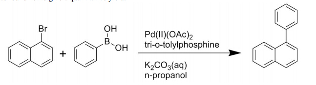
McFarlane J, Luo H, Garland M, et al. (2010) Evaluation of phenylnaphthalenes as heat transfer fluids for high temperature energy applications. Sep Sci Technol 45: 1908-1920. doi: 10.1080/01496395.2010.493800
|
| [27] |
Steele WV, Chirico RD, Knipmeyer SE, et al. (1992) The thermodynamic properties of 9-methylcarbazole and of 1,2,3,4-tetrahydro-9-methylcarbazole. J Chem Therm 24: 245-271. doi: 10.1016/S0021-9614(05)80066-7
|
| [28] |
Zalba B, Marın JM, Cabeza LF, et al. (2003) Review on thermal energy storage with phase change: materials, heat transfer analysis and applications. App Thermal Eng 23: 251-283. doi: 10.1016/S1359-4311(02)00192-8
|
| [29] |
Wilhelms A, Telnæs N, Steen A, et al. (1998) A quantitative study of aromatic hydrocarbons in a natural maturity shale sequence—the 3-methylphenanthrene/retene ratio, a pragmatic maturity parameter. Org Geochem 29: 97-105. doi: 10.1016/S0146-6380(98)00112-0
|
| [30] |
Orem WH, Tatu CA, Lerch HE, et al. (2007) Organic compounds in produced waters from coalbed natural gas wells in the Powder River Basin, Wyoming, USA. App Geochem 22: 2240-2256. doi: 10.1016/j.apgeochem.2007.04.010
|
| [31] |
Miyaura M, Yamada K, Suzuki A (1979) A new stereospecific cross-coupling by the palladium-catalyzed reaction of 1-alkenylboranes with 1-alkenyl or 1-alkynyl halides. Tet Lett 20: 3437-3440. doi: 10.1016/S0040-4039(01)95429-2
|
| [32] |
Eguchi H, Nishiyama M, Ishikawa S, et al. (2012) Development and industrialization of efficient cross-coupling reactions. J Syn Org Chem Japan 70: 937-946. doi: 10.5059/yukigoseikyokaishi.70.937
|
| [33] |
Franzen R, Xu YJ (2005) Review on green chemistry - Suzuki cross coupling in aqueous media. Can J Chem 83: 266-272. doi: 10.1139/v05-048
|
| [34] |
Narayanan R (2010) Recent advances in noble metal nanocatalysts for Suzuki and Heck cross-coupling reactions. Molecules 15: 2124-2138. doi: 10.3390/molecules15042124
|
| [35] |
Polshettiwar V, Decottignies A, Len C, et al. (2010) Suzuki-Miyaura cross-coupling reactions in aqueous media: Green and sustainable syntheses of biaryls. ChemSusChem 3: 502-522. doi: 10.1002/cssc.200900221
|
| [36] |
Seechurn C, Kitching MO, Colacot TJ, et al. (2012) Palladium-catalyzed cross-coupling: A historical contextual perspective to the 2010 Nobel prize. Angew Chem 51: 5062-5085. doi: 10.1002/anie.201107017
|
| [37] |
Colon I, Kelsey DR (1986) Coupling of aryl chlorides by nickel and reducing metals. J Org Chem 51: 2627-2637. doi: 10.1021/jo00364a002
|
| [38] | Bell JR, Joseph RAI, McFarlane J, et al. (2012) Phenylnaphthalene as a Heat Transfer Fluid for Concentrating Solar Power: High-Temperature Static Experiments Oak Ridge, TN: Oak Ridge National Laboratory. ORNL/TM-2012/118. |
| [39] |
Cioslowski J, Liu G, Martinov M, et al. (1996) Energetics and site specificity of the homolytic C-H bond cleavage in benzenoid hydrocarbons: An ab initio electronic structure study. J Am Chem Soc 118: 5261-5264. doi: 10.1021/ja9600439
|
| [40] |
Cioslowski J, Piskorz P, Liu G, et al. (1996) Regularities in energies and geometries of biaryls: An ab initio electronic structure study. J Phys Chem 100: 19333-19335. doi: 10.1021/jp961298b
|
| [41] |
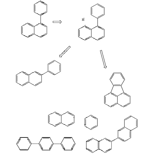
Cioslowski J, Piskorz P, Moncrieff D (1998) Thermally induced cyclodehydrogenation of biaryls: A simple radical reaction of a sequence of rearrangements? J Org Chem 63: 4051-4054. doi: 10.1021/jo980132z
|
| [42] |
Gaynor S, Greszta D, Mardare D, et al. (1994) Controlled radical polymerization. J Macromolec Sci, Part A: Pure Appl Chem 31: 1561-1578. doi: 10.1080/10601329408545868
|
| [43] |
Duran A, Carmona M, Monteagudo JM (2004) Modelling soot and SOF emissions from a diesel engine. Chemosphere 56: 209-225. doi: 10.1016/j.chemosphere.2004.03.008
|
| [44] |
Pope CJ, Marr JA, Howard JB (1993) Chemistry of fullerenes C60 and C70 formation in flames. J Phys Chem 97: 11001-11013. doi: 10.1021/j100144a018
|
| [45] | MatLab (2012). 2012a ed. Natick, MA: Mathworks. |
| [46] | Hines AL, Maddox RN (1985) Mass Transfer Fundamentals and Applications. Englewood Cliffs, NJ: Prentice-Hall, Inc |
| [47] |
Rocha MAA, Lima CFRAC, Santos LMNBF (2008) Phase transition thermodynamics of phenyl and biphenyl naphthalenes. J Chem Thermodyn 40: 1458-1463. doi: 10.1016/j.jct.2008.04.010
|
| [48] | Turchi C (2010) Parabolic Trough Reference Plant for Cost Modeling with Solar Advisor Model (SAM). Golden, CO: National Renewable Energy Laboratory. NREL/TP-550-47605. |
| [49] |
Curzon FL, Ahlborn B (1975) Efficiency of a Carnot engine at maximum power output. Am J Phys 43: 22-24. doi: 10.1119/1.10023
|
| [50] | Kolb GJ, Diver RB (2008) Conceptual design of an advanced trough utilizing a molten salt working fluid. SolarPACES Symposium. Las Vegas, NV: Sandia National Laboratories, Albuquerque, NM. |
| [51] | Kennedy CE, Price H (2005) Progress in development of high-temperature solar-selective coating. International Solar Energy Conference. Orlando, FL: National Renewable Energy Laboratory. pp. ISEC2005-76039. |
| [52] |
Adili A, Kerkeni C, Ben Nasralla S (2009) Estimation of thermophysical properties of fouling using inverse problem and its impact on heat transfer efficiency. Solar Energy 83: 1619-1628. doi: 10.1016/j.solener.2009.05.014
|
| [53] | Kennedy CE, Price H (2005) Progress in Development of High-Temperature Solar-Selective Coating. Golden, CO National Renewable Energy Laboratory. NREL/CP-520-36997. |
| [54] | Kennedy CE (2002) Review of Mid-to-High-Temperature Solar Selective Absorber Materials. Golden, CO National Renewable Energy Laboratory. NREL/TP-520-31267. |
Figures(14) / Tables(9)

Joanna McFarlane, Jason Richard Bell, David K. Felde, Robert A. Joseph III, A. Lou Qualls, Samuel Paul Weaver. Performance and Thermal Stability of a Polyaromatic Hydrocarbon in a Simulated Concentrating Solar Power Loop[J]. AIMS Energy, 2014, 2(1): 41-70. doi: 10.3934/energy.2014.1.41


 DownLoad: