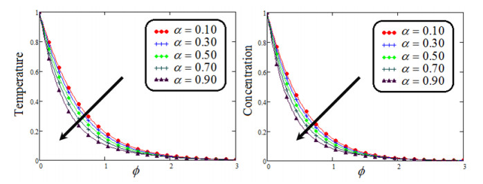
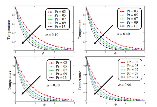
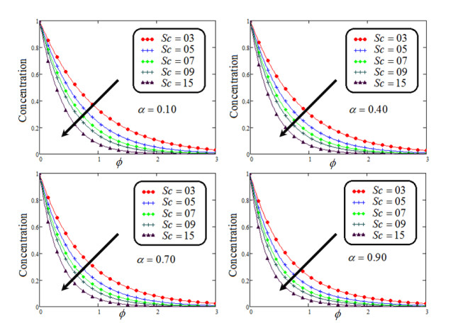
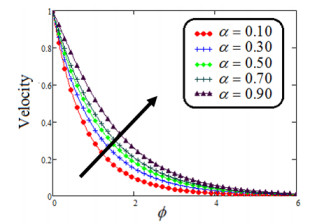
A new approach is used to investigate the analytical solutions of the mathematical fractional Casson fluid model that is described by the Constant Proportional Caputo fractional operator having non-local and singular kernel near an infinitely vertical plate. The phenomenon has been expressed in terms of partial differential equations, and the governing equations were then transformed in non-dimensional form. For the sake of generalized memory effects, a new mathematical fractional model is formulated based on the newly introduced Constant Proportional Caputo fractional derivative operator. This fractional model has been solved analytically, and exact solutions for dimensionless velocity, concentration and energy equations are calculated in terms of Mittag-Leffler functions by employing the Laplace transformation method. For the physical significance of various system parameters such as $ \alpha $, $ \beta $, $ Pr $, $ Gr $, $ Gm $, $ Sc $ on velocity, temperature and concentration profiles, different graphs are demonstrated by Mathcad software. The Constant Proportional Caputo fractional parameter exhibited a retardation effect on momentum and energy profile, but it is visualized that for small values of Casson fluid parameter, the velocity profile is higher. Furthermore, to validated the acquired solutions, some limiting models such as the ordinary Newtonian model are recovered from the fractionalized model. Moreover, the graphical representations of the analytical solutions illustrated the main results of the present work. Also, from the literature, it is observed that to deriving analytical results from fractional fluid models developed by the various fractional operators is difficult, and this article contributes to answering the open problem of obtaining analytical solutions for the fractionalized fluid models.
Citation: Aziz Ur Rehman, Muhammad Bilal Riaz, Ilyas Khan, Abdullah Mohamed. Time fractional analysis of Casson fluid with application of novel hybrid fractional derivative operator[J]. AIMS Mathematics, 2023, 8(4): 8185-8209. doi: 10.3934/math.2023414
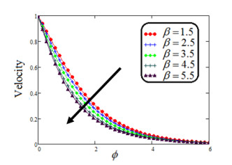
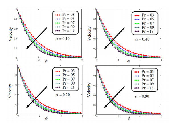
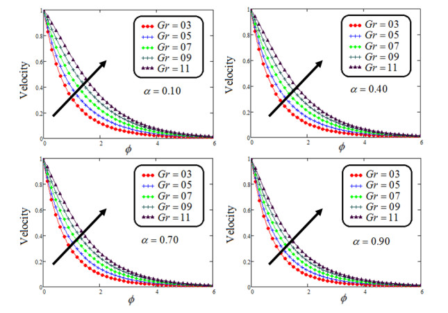
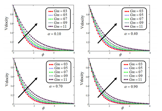
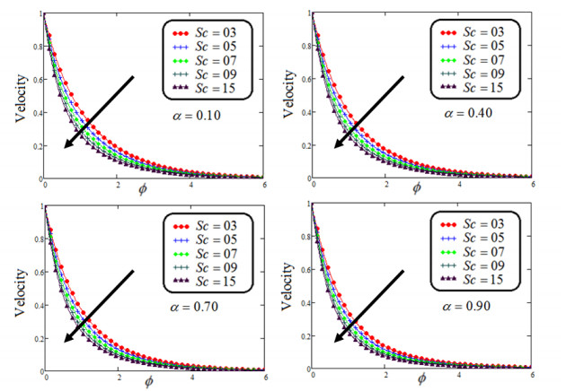
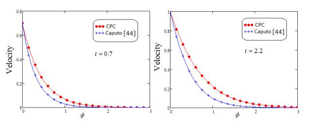
A new approach is used to investigate the analytical solutions of the mathematical fractional Casson fluid model that is described by the Constant Proportional Caputo fractional operator having non-local and singular kernel near an infinitely vertical plate. The phenomenon has been expressed in terms of partial differential equations, and the governing equations were then transformed in non-dimensional form. For the sake of generalized memory effects, a new mathematical fractional model is formulated based on the newly introduced Constant Proportional Caputo fractional derivative operator. This fractional model has been solved analytically, and exact solutions for dimensionless velocity, concentration and energy equations are calculated in terms of Mittag-Leffler functions by employing the Laplace transformation method. For the physical significance of various system parameters such as $ \alpha $, $ \beta $, $ Pr $, $ Gr $, $ Gm $, $ Sc $ on velocity, temperature and concentration profiles, different graphs are demonstrated by Mathcad software. The Constant Proportional Caputo fractional parameter exhibited a retardation effect on momentum and energy profile, but it is visualized that for small values of Casson fluid parameter, the velocity profile is higher. Furthermore, to validated the acquired solutions, some limiting models such as the ordinary Newtonian model are recovered from the fractionalized model. Moreover, the graphical representations of the analytical solutions illustrated the main results of the present work. Also, from the literature, it is observed that to deriving analytical results from fractional fluid models developed by the various fractional operators is difficult, and this article contributes to answering the open problem of obtaining analytical solutions for the fractionalized fluid models.

| [1] |
M. Kahshan, D. Lu, A. M. Siddiqui, A Jeffrey fluid model for a porous-walled channel: application to flat plate dialyzer, Sci. Rep., 9 (2019), 15879. https://doi.org/10.1038/s41598-019-52346-8 doi: 10.1038/s41598-019-52346-8

|
| [2] |
R. Mohebbi, A. A. Delouei, A. Jamali, M. Izadi, A. A. Mohamad, Pore-scale simulation of non-Newtonian power-law fluid flow and forced convection in partially porous media: thermal lattice Boltzmann method, Phys. A., 525 (2019), 642–656. https://doi.org/10.1016/j.physa.2019.03.039 doi: 10.1016/j.physa.2019.03.039
|
| [3] |
A. U. Rehman, M. B. Riaz, S. T. Saeed, S. Yao, Dynamical analysis of radiation and heat transfer on MHD second grade fluid, Comp. Model. Eng. Sci., 129 (2021), 689–703. https://doi.org/10.32604/cmes.2021.014980 doi: 10.32604/cmes.2021.014980
|
| [4] |
M. B. Riaz, K. A. Abro, K. M. Abualnaja, A. Akgül, A. U. Rehman, M. Abbas, et al., Exact solutions involving special functions for unsteady convective flow of magnetohydrodynamic second grade fluid with ramped conditions, Adv. Differ. Equ., 2021 (2021), 408. https://doi.org/10.1186/s13662-021-03562-y doi: 10.1186/s13662-021-03562-y
|
| [5] |
M. B. Riaz, J. Awrejcewicz, A. U. Rehman, Functional effects of permeability on Oldroyd-B fluid under magnetization: a comparison of slipping and non-slipping solutions, Appl. Sci., 11 (2021), 11477. https://doi.org/10.3390/app112311477 doi: 10.3390/app112311477
|
| [6] |
Z. Khan, N. Tairan, W. K. Mashwani, H. U. Rasheed, H. Shah, W. Khan, MHD and slip effect on two-immiscible third grade fluid on thin film flow over a vertical moving belt, Open Phys., 17 (2019), 575–586. https://doi.org/10.1515/phys-2019-0059 doi: 10.1515/phys-2019-0059
|
| [7] | N. Casson, A flow equation for pigment-oil suspensions of the printing ink type, In: Rheology of disperse systems, Pergamon Press, 1959, 84–104. |
| [8] |
R. K. Dash, K. N. Mehta, G. Jayaraman, Casson fluid flow in a pipe filled with a homogeneous porous medium, Int. J. Eng. Sci., 34 (1996), 1145–1156. https://doi.org/10.1016/0020-7225(96)00012-2 doi: 10.1016/0020-7225(96)00012-2
|
| [9] | Y. C. Fung, Biodynamics, Circulation, New York: Springer-Verlag, 1984. https://doi.org/10.1007/978-1-4757-3884-1 |
| [10] |
A. Khalid, I. Khan, A. Khan, S. Shafie, Unsteady MHD free convection flow of Casson fluid past over an oscillating vertical plate embedded in a porous medium, Eng. Sci. Technol. Int. J., 18 (2015), 309–317. https://doi.org/10.1016/j.jestch.2014.12.006 doi: 10.1016/j.jestch.2014.12.006
|
| [11] |
K. Bhattacharyya, T. Hayat, A. Alsaedi, Analytic solution for magnetohydrodynamic boundary layer flow of Casson fluid over a stretching/shrinking sheet with wall mass transfer, Chin. Phys. B, 22 (2013), 024702. https://doi.org/10.1088/1674-1056/22/2/024702 doi: 10.1088/1674-1056/22/2/024702
|
| [12] |
S. Oka, An approach to $\alpha$ unified theory of the flow behaviour of time-independent non-Newtonian suspensions, Jpn. J. Appl. Phys., 10 (1971), 287. https://doi.org/10.1143/JJAP.10.287 doi: 10.1143/JJAP.10.287
|
| [13] |
A. V. Mernone, J. N. Mazumdar, S. K. Lucas, A mathematical study of peristaltic transport of a Casson fluid, Math. Comput. Model., 35 (2022), 895–912. https://doi.org/10.1016/S0895-7177(02)00058-4 doi: 10.1016/S0895-7177(02)00058-4
|
| [14] | E. M. Arthur, I. Y. Seini, L. B. Bortteir, Analysis of Casson fluid flow over a vertical porous surface with chemical reaction in the presence of magnetic field, J. Appl. Math. Phys., 3 (2015), 713–723. |
| [15] |
K. U. Rehman, E. A. Algehyne, F. Shahzad, E. M. Sherif, Y. M. Chu, On thermally corrugated porous enclosure (TCPE) equipped with Casson liquid suspension: finite element thermal analysis, Case Stud. Therm. Eng., 25 (2021), 100873. https://doi.org/10.1016/j.csite.2021.100873 doi: 10.1016/j.csite.2021.100873
|
| [16] |
Q. Lou, B. Ali, S. U. Rehman, D. Habib, S. Abdal, N. A. Shah, et al., Micropolar dusty fluid: coriolis force effects on dynamics of MHD rotating fluid when Lorentz force is significant, Mathematics, 10 (2022), 2630. https://doi.org/10.3390/math10152630 doi: 10.3390/math10152630
|
| [17] |
M. Z. Ashraf, S. U. Rehman, S. Farid, A. K. Hussein, B. Ali, N. A. Shah, et al., Insight into significance of bioconvection on MHD tangent hyperbolic nanofluid flow of irregular thickness across a slender elastic surface, Mathematics, 10 (2022), 2592. https://doi.org/10.3390/math10152592 doi: 10.3390/math10152592
|
| [18] |
J. K. Madhukesh, R. N. Kumar, R. J. P. Gowda, B. C. Prasannkumara, G. K. Ramesh, M. I. Khan, et al., Numerical simulation of AA7072-AA7075/water-based hybrid nanofluid flow over a curved stretching sheet with Newtonian heating: a non-Fourier heat flux model approach, J. Mol. Liq., 335 (2021), 116103. https://doi.org/10.1016/j.molliq.2021.116103 doi: 10.1016/j.molliq.2021.116103
|
| [19] |
A. Bagh, S. Anum, S. Imran, A. Qasem, J. Fahd, Significance of suction/injection, gravity modulation, thermal radiation, and magnetohydrodynamic on dynamics of micropolar fluid subject to an inclined sheet via finite element approach, Case Stud. Therm. Eng., 28 (2021), 101537. https://doi.org/10.1016/j.csite.2021.101537 doi: 10.1016/j.csite.2021.101537
|
| [20] |
Q. Raza, M. Z. A. Qureshi, B. A. Khan, A. K. Hussein, B. Ali, N. A. Shah, et al., Insight into dynamic of Mono and hybrid Nanofluids subject to binary chemical reaction, activation energy, and magnetic field through the porous surfaces, Mathematics, 10 (2022), 3013. https://doi.org/10.3390/math10163013 doi: 10.3390/math10163013
|
| [21] |
M. Mustafa, T. Hayat, I. Pop, A. Aziz, Unsteady boundary layer flow of a Casson fluid due to an impulsively started moving flat plate, Heat Transf., 40 (2011), 563–576. https://doi.org/10.1002/htj.20358 doi: 10.1002/htj.20358
|
| [22] |
A. Bagh, T. Thirupathi, H. Danial, S. Nadeem, R. Saleem, Finite element analysis on transient MHD 3D rotating flow of Maxwell and tangent hyperbolic nanofluid past a bidirectional stretching sheet with Cattaneo Christov heat flux model, Case Stud. Therm. Eng., 28 (2022), 101089. https://doi.org/10.1016/j.tsep.2021.101089 doi: 10.1016/j.tsep.2021.101089
|
| [23] |
M. Z. A. Qureshi, M. Faisal, Q. Raza, B. Ali, T. Botmart, N. A. Shah, Morphological nanolayer impact on hybrid nanofluids flow due to dispersion of polymer/CNT matrix nanocomposite material, AIMS Math., 8 (2023), 633–656. https://doi.org/10.3934/math.2023030 doi: 10.3934/math.2023030
|
| [24] |
B. Ali, S. Imran, A. Ali, S. Norazak, A. Liaqat, H. Amir, Significance of Lorentz and Coriolis forces on dynamics of water based silver tiny particles via finite element simulation, Ain Sha. Eng. J., 13 (2022), 101572. https://doi.org/10.1016/j.asej.2021.08.014 doi: 10.1016/j.asej.2021.08.014
|
| [25] |
S. Pramanik, Casson fluid flow and heat transfer past an exponentially porous stretching surface in presence of thermal radiation, Ain Shams Eng. J., 5 (2014), 205–212. https://doi.org/10.1016/j.asej.2013.05.003 doi: 10.1016/j.asej.2013.05.003
|
| [26] |
M. S. Osman, A. Korkmaz, H. Rezazadeh, M. Mirzazadeh, M. Eslami, Q. Zhou, The unified method for conformable time fractional Schrödinger equation with perturbation terms, Chin. J. Phys., 56 (2018), 2500–2506. https://doi.org/10.1016/j.cjph.2018.06.009 doi: 10.1016/j.cjph.2018.06.009
|
| [27] | M. Al-Smadi, A. Freihat, O. A. Arqub, N. Shawagfeh, A novel multistep generalized differential transform method for solving fractional-order Lu chaotic and hyperchaotic systems, J. Comput. Anal. Appl., 19 (2015), 713–724. |
| [28] |
S. Momani, A. Freihat, M. Al-Smadi, Analytical study of fractional-order multiple chaotic Fitzhugh-Nagumo neurons model using multistep generalized differential transform method, Abstr. Appl. Anal., 2014 (2014), 276279. https://doi.org/10.1155/2014/276279 doi: 10.1155/2014/276279
|
| [29] |
M. Alabedalhadi, M. Al-Smadi, S. Al-Omari, D. Baleanu, S. Momani, Structure of optical soliton solution for nonliear resonant space-time Schrödinger equation in conformable sense with full nonlinearity term, Phys. Scr., 95 (2020), 105215. https://doi.org/10.1088/1402-4896/abb739 doi: 10.1088/1402-4896/abb739
|
| [30] | Z. Altawallbeh, M. Al-Smadi, I. Komashynska, A. Ateiwi, Numerical solutions of fractional systems of two-point BVPs by using the iterative reproducing kernel algorithm, Ukr. Math. J., 70 (2018), 687–701. |
| [31] |
M. Al-Smadi, N. Djeddi, S. Momani, S. Al-Omari, S. Araci, An attractive numerical algorithm for solving nonlinear Caputo-Fabrizio fractional Abel differential equation in a Hilbert space, Adv. Differ. Equ., 2021 (2021), 271. https://doi.org/10.1186/s13662-021-03428-3 doi: 10.1186/s13662-021-03428-3
|
| [32] |
M. N. Islam, M. A. Akbar, Closed form exact solutions to the higher dimensional fractional Schrodinger equation via the modified simple equation method, J. Appl. Math. Phys., 6 (2018), 90–102. https://doi.org/10.4236/jamp.2018.61009 doi: 10.4236/jamp.2018.61009
|
| [33] |
M. Al-Smadi, O. A. Arqub, S. Hadid, Approximate solutions of nonlinear fractional Kundu-Eckhaus and coupled fractional massive Thirring equations emerging in quantum field theory using conformable residual power series method, Phys. Scr., 95 (2020), 105205. https://doi.org/10.1088/1402-4896/abb420 doi: 10.1088/1402-4896/abb420
|
| [34] |
M. Al-Smadi, O. A. Arqub, M. Gaith, Numerical simulation of telegraph and Cattaneo fractional-type models using adaptive reproducing kernel framework, Math. Methods Appl. Sci., 44 (2021), 8472–8489. https://doi.org/10.1002/mma.6998 doi: 10.1002/mma.6998
|
| [35] |
S. Momani, N. Djeddi, M. Al-Smadi, S. Al-Omari, Numerical investigation for Caputo-Fabrizio fractional Riccati and Bernoulli equations using iterative reproducing kernel method, Appl. Numer. Math., 170 (2021), 418–434. https://doi.org/10.1016/j.apnum.2021.08.005 doi: 10.1016/j.apnum.2021.08.005
|
| [36] |
S. Hasan, M. Al-Smadi, A. El-Ajou, S. Momani, S. Hadid, Z. Al-Zhour, Numerical approach in the Hilbert space to solve a fuzzy Atangana-Baleanu fractional hybrid system, Chaos Solitons Fract., 143 (2021), 110506. https://doi.org/10.1016/j.chaos.2020.110506 doi: 10.1016/j.chaos.2020.110506
|
| [37] |
M. B. Riaz, J. Awrejcewicz, A. U. Rehman, M. Abbas, Special functions-based solutions of unsteady convective flow of a MHD Maxwell fluid for ramped wall temperature and velocity with concentration, Adv. Differ. Equ., 2021 (2021), 500. https://doi.org/10.1186/s13662-021-03657-6 doi: 10.1186/s13662-021-03657-6
|
| [38] |
M. B. Riaz, J. Awrejcewicz, A. U. Rehman, A. Akgül, Thermophysical investigation of Oldroyd-b fluid with functional effects of permeability: memory effect study using non-singular kernel derivative approach, Fractal Fract., 5 (2021), 124. https://doi.org/10.3390/fractalfract5030124 doi: 10.3390/fractalfract5030124
|
| [39] | A. Atangana, D. Baleanu, New fractional derivative with non local and non-singular kernel: theory and application to heat transfer model, Thermal Sci., 20 (2016), 763–769. |
| [40] |
A. U. Rehman, J. Awrejcewicz, M. B. Riaz, F. Jarad, Mittag-Leffler form solutions of natural convection flow of second grade fluid with exponentially variable temperature and mass diffusion using Prabhakar fractional derivative, Case Stud. Therm. Eng., 34 (2022), https://doi.org/10.1016/j.csite.2022.102018 doi: 10.1016/j.csite.2022.102018
|
| [41] |
M. B. Riaz, A. U. Rehman, J. Awrejcewicz, A. Akgül, Power law kernel analysis of MHD Maxwell fluid with ramped boundary conditions: transport phenomena solutions based on special functions, Fractal Fract., 5 (2021), 248. https://doi.org/10.3390/fractalfract5040248 doi: 10.3390/fractalfract5040248
|
| [42] |
A. U. Rehman, M. B. Riaz, W. Rehman, J. Awrejcewicz, D. Baleanu, Fractional modeling of viscous fluid over a moveable inclined plate subject to exponential heating with singular and non-singular kernels, Math. Comput. Appl., 27 (2022), 8. https://doi.org/10.3390/mca27010008 doi: 10.3390/mca27010008
|
| [43] |
Y. M. Chu, R. Ali, M. I. Asjad, A. Ahmadian, N. Senu, Heat transfer flow of Maxwell hybrid nanofluids due to pressure gradient into rectangular region, Sci. Rep., 10 (2020), 16643. https://doi.org/10.1038/s41598-020-73174-1 doi: 10.1038/s41598-020-73174-1
|
| [44] |
N. Sene, Analytical solutions of a class of fluids models with the Caputo fractional derivative, Fractal Fract., 6 (2022), 35. https://doi.org/10.3390/fractalfract6010035 doi: 10.3390/fractalfract6010035
|
| [45] |
T. Hayat, S. A. Shehzad, A. Alsaedi, M. S. Alhothuali, Mixed convection stagnation point flow of Casson fluid with convective boundary conditions, Chin. Phys. Lett., 29 (2012), 114704. https://doi.org/10.1088/0256-307X/29/11/114704 doi: 10.1088/0256-307X/29/11/114704
|
| [46] |
K. B. Charyya, Boundary layer stagnation-point flow of Casson fluid and heat transfer towards a shrinking/stretching sheet, Front. Heat Mass Tran., 4 (2013), 023003. http://dx.doi.org/10.5098/hmt.v4.2.3003 doi: 10.5098/hmt.v4.2.3003
|
| [47] |
A. Khalid, I. Khan, A. Khan, S. Shafie, Unsteady MHD free convection flow of Casson fluid past over an oscillating vertical plate embedded in a porous medium, Eng. Sci. Technol. Int. J., 18 (2015), 309–317. https://doi.org/10.1016/j.jestch.2014.12.006 doi: 10.1016/j.jestch.2014.12.006
|
| [48] |
M. Mustafa, J. A. Khan, Model for flow of Casson nanofluid past a non-linearly stretching sheet considering magnetic field effects, AIP Adv., 5 (2015), 077148. https://doi.org/10.1063/1.4927449 doi: 10.1063/1.4927449
|
| [49] |
D. Baleanu, A. Fernandez, A. Akgül, On a fractional operator combining Proportional and Classical Differintegrals, Mathematics, 8 (2020), 360. https://doi.org/10.3390/math8030360 doi: 10.3390/math8030360
|

Figures(11)

Aziz Ur Rehman, Muhammad Bilal Riaz, Ilyas Khan, Abdullah Mohamed. Time fractional analysis of Casson fluid with application of novel hybrid fractional derivative operator[J]. AIMS Mathematics, 2023, 8(4): 8185-8209. doi: 10.3934/math.2023414


 DownLoad: