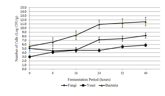
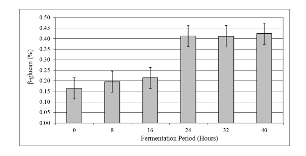
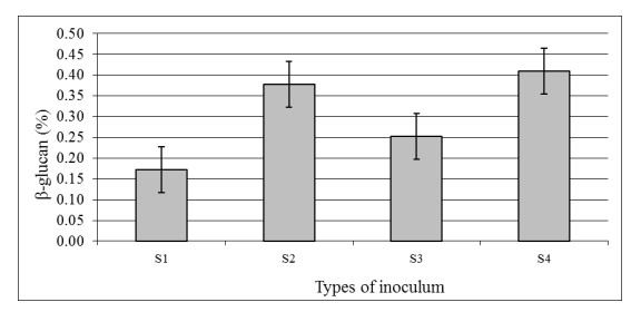
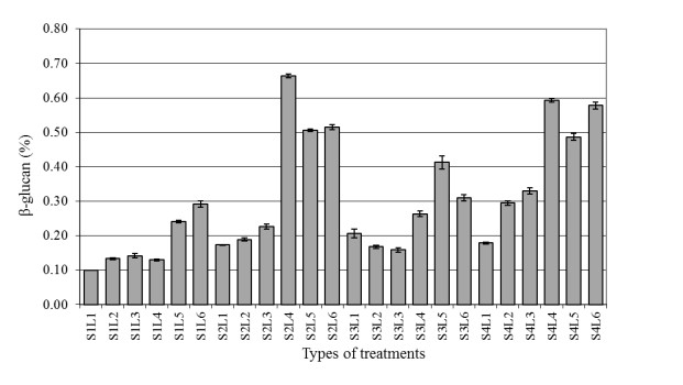
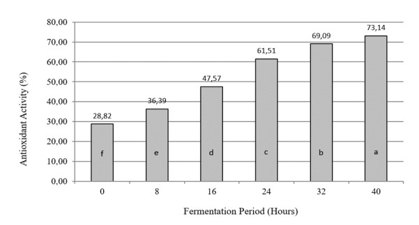
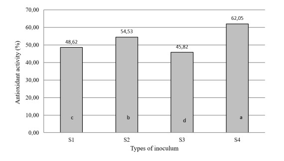
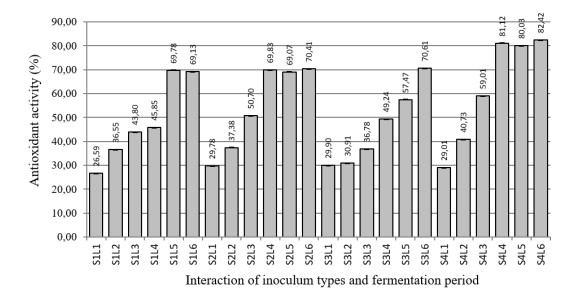
The aim of the research was to study the effect of inoculum type and fermentation time on microbial growth patterns (yeast, fungi and bacteria), β-glucan formation and antioxidant activity during soybean fermentation into tempe. The research was conducted using factorial Completely Randomized Block Design with 3 replications. The first factor was the types of inoculum: commercial inoculum of tempe, Raprima (3%), a single inoculum of S. cerevisiae (3%), a single inoculum of R. oligosporus (3%), and mixed inoculum of 1.5% S. cerevisiae and 1.5% R. oligosporus. The second factor was the length of fermentation which consisted of 0, 8, 16, 24, 32 and 40 hours at room temperature. Regarding the number of fungi, yeasts and bacteria, the observational data were presented descriptively in the form of graphs, while for the data from the analysis of β-glucan and antioxidant activity, the data obtained were analyzed for variance with analysis of variance (ANOVA) and then analyzed further by the Least Significant Difference (LSD) at the 5% significance level. The results showed that the type of inoculum and duration of fermentation had an effect on increasing the growth of fungi, yeasts and bacteria, as well as increasing β-glucan content and the antioxidant activity of tempe. Yeast growth had a more dominant effect on increasing β-glucan content and antioxidant activity compared to fungi and bacteria. Tempe inoculated with a mixed inoculum of 1.5% R. oligosporus + 1.5% S. cerevisiae, resulted in the highest β-glucan content of 0.58% and the highest antioxidant activity at 82.42%. In conclusion, a mixed inoculum of 1.5% R. oligosporus + 1.5% S. cerevisiae with 36−40 hours of fermentation produced tempe with the highest β-glucan content and antioxidant activity. Therefore, the β-glucan content causes tempe to have better potential health benefits than tempe without the addition of S. cerevisiae.
Citation: Samsul Rizal, Maria Erna Kustyawati, Murhadi, Udin Hasanudin, Subeki. The effect of inoculum types on microbial growth, β-glucan formation and antioxidant activity during tempe fermentation[J]. AIMS Agriculture and Food, 2022, 7(2): 370-386. doi: 10.3934/agrfood.2022024
The aim of the research was to study the effect of inoculum type and fermentation time on microbial growth patterns (yeast, fungi and bacteria), β-glucan formation and antioxidant activity during soybean fermentation into tempe. The research was conducted using factorial Completely Randomized Block Design with 3 replications. The first factor was the types of inoculum: commercial inoculum of tempe, Raprima (3%), a single inoculum of S. cerevisiae (3%), a single inoculum of R. oligosporus (3%), and mixed inoculum of 1.5% S. cerevisiae and 1.5% R. oligosporus. The second factor was the length of fermentation which consisted of 0, 8, 16, 24, 32 and 40 hours at room temperature. Regarding the number of fungi, yeasts and bacteria, the observational data were presented descriptively in the form of graphs, while for the data from the analysis of β-glucan and antioxidant activity, the data obtained were analyzed for variance with analysis of variance (ANOVA) and then analyzed further by the Least Significant Difference (LSD) at the 5% significance level. The results showed that the type of inoculum and duration of fermentation had an effect on increasing the growth of fungi, yeasts and bacteria, as well as increasing β-glucan content and the antioxidant activity of tempe. Yeast growth had a more dominant effect on increasing β-glucan content and antioxidant activity compared to fungi and bacteria. Tempe inoculated with a mixed inoculum of 1.5% R. oligosporus + 1.5% S. cerevisiae, resulted in the highest β-glucan content of 0.58% and the highest antioxidant activity at 82.42%. In conclusion, a mixed inoculum of 1.5% R. oligosporus + 1.5% S. cerevisiae with 36−40 hours of fermentation produced tempe with the highest β-glucan content and antioxidant activity. Therefore, the β-glucan content causes tempe to have better potential health benefits than tempe without the addition of S. cerevisiae.

| [1] |
Bintari SH, Anisa DP, Veronika EJ, et al. (2008) Effect inoculation of Micrococcus luteus to growth of mold and content isoflavone at tempe processing. Biosaintifika: J Bio Bio Edu 1: 1–8. https://doi.org/10.15294/biosaintifika.v1i1.43 doi: 10.15294/biosaintifika.v1i1.43

|
| [2] | Roubous HPJ, Nout MJR (2011) Anti-diarrhoeal aspect of fermented soya beans, In: El-Shemy H. (Eds), Soybean and Health, London: Intech Open, 383–406. |
| [3] |
Kustyawati ME (2009) Study on the role of yeast in tempe production. Agritech 29: 64–70. https://doi.org/10.22146/agritech.9765 doi: 10.22146/agritech.9765
|
| [4] | Nurdini AL, Nuraida L, Suwanto A, et al. (2015) Microbial growth dynamics during tempe fermentation in two different home industries. Food Res Int 22: 1668–1674. |
| [5] | Astawan M, Wresdiyati T, Widowati S, et al. (2013) Phsyco-chemical characteristics and functional properties of tempeh made from different soybeans varieties. Pangan 22: 241–252. |
| [6] |
Mambang DEP, Rosidah, Suryanto D (2014) Antibacterial activity of tempe extracts on Bacillus subtilis and Staphylococcus aureus. J Teknol dan Industri Pangan 25: 115–118. https://doi.org/10.6066/jtip.2014.25.1.115 doi: 10.6066/jtip.2014.25.1.115
|
| [7] |
Virgianti DP (2015) Uji antagonis jamur tempe (Rhizopus sp.) terhadap bakteri patogen enterik. Majalah Ilmiah Biologi Biosfera: A Sci J 32: 162–168. https://doi.org/10.20884/1.mib.2015.32.3.339 doi: 10.20884/1.mib.2015.32.3.339
|
| [8] |
Kuligowski M, Kuligowska IJ, Nowak J (2013) Evaluation of bean and soy tempeh influence on intestinal bacteria and estimation of antibacterial properties of bean tempeh. Pol J Microbiol 62: 189–194. https://doi.org/10.33073/pjm-2013-024 doi: 10.33073/pjm-2013-024
|
| [9] |
Pengkumsri N, Sivamaruthi BS, Sirilun S, et al. (2017) Extraction of β-glukan from Saccharomyces cerevisiae: Comparison of different extraction methods and in vivo assessment of immunomodulatory effect in mice. Food Sci Tech 37: 124–130. https://doi.org/10.1590/1678-457X.10716 doi: 10.1590/1678-457X.10716
|
| [10] | Hetland G, Johnson E, Eide DM, et al. (2013) Antimicrobial effects of β-glucans and pectin and of the Agaricus blazei-based mushroom extract, AndoSanTM. Examples of mouse models for pneumococcal, fecal bacterial, and mycobacterial infections. Microb Pathog Strategies Combating Them: Sci, Technol Edu 1: 889–898. |
| [11] |
Rizal S, Kustyawati ME (2019) Characteristics of sensory and Beta-glucan content of soybean tempe with addition of Saccharomyces cerevisiae. J Teknol Pertanian 20: 127–138. https://doi.org/10.21776/ub.jtp.2019.020.02.6 doi: 10.21776/ub.jtp.2019.020.02.6
|
| [12] |
Rizal S, Kustyawati ME, Murhadi, et al. (2020) Growth optimization of Saccharomyces cerevisiae and Rhizopus oligosporus during fermentation to produce tempe with high β-glucan content. Biodiversitas J Biol Diversity 21: 2667–2673. https://doi.org/10.13057/biodiv/d210639 doi: 10.13057/biodiv/d210639
|
| [13] |
Rizal S, Kustyawati ME, Murhadi, et al. (2021) The growth of yeast and fungi, the formation of β-glucan, and the antibacterial activities during soybean fermentation in producing tempe. Int J Food Sci. 6: 1–8. https://doi.org/10.1155/2021/6676042 doi: 10.1155/2021/6676042
|
| [14] |
Rizal S, Kustyawati ME, Suharyono, et al. (2022) Changes of nutritional composition of tempeh during fermentation with the addition of Saccharomyces cerevisiae. Biodiversitas J Biol Diversity 23: 1553–1559. https://doi.org/10.13057/biodiv/d230345 doi: 10.13057/biodiv/d230345
|
| [15] | Rizal S, Kustyawati ME, Murhadi, et al. (2018) Pengaruh konsentrasi Saccharomyces cerevisiae pada kandungan abu, protein, lemak dan β-glukan tempe. Prosiding Seminar Nasional Fakultas Pertanian UNS 2: 96–103. |
| [16] |
Kustyawati ME, Subeki, Murhadi, et al. (2020) Vitamin B12 production in soybean fermentation for tempeh. AIMS Agric Food 5: 262–271. https://doi.org/10.3934/agrfood.2020.2.262 doi: 10.3934/agrfood.2020.2.262
|
| [17] |
Bavia ACF, Silva CE, Ferreira MP, et al. (2012) Chemical composition of tempeh from soybean cultivars specially developed for human consumption. Food Sci Tech 32: 613–620. https://doi.org/10.1590/S0101-20612012005000085 doi: 10.1590/S0101-20612012005000085
|
| [18] |
Kusmiati, Tamat SR, Jusuf E, et al. (2007) Beta-glucan production from two strains of Agrobacterium sp. in medium containing of molases and uracil combine. Biodiversivitas 8: 253–256. https://doi.org/10.13057/biodiv/d080210 doi: 10.13057/biodiv/d080210
|
| [19] |
Ismail J, Runtuwene MRJ, Fatimah F (2012) Total phenolic compounds and antioxidant activity of the seed and skin of pinang yaki (areca vestiaria giseke) fruits (Areca vetiaria Giseke). J Ilmiah Sains 12: 84–85. https://doi.org/10.35799/jis.12.2.2012.557 doi: 10.35799/jis.12.2.2012.557
|
| [20] |
Moreno MRF, Leisner JJ, Tee LK, et al. (2002) Microbial analysis of Malaysian tempeh, and characterization of two bacteriocins produced by isolates of Enterococcus faecium. J Appl Microbiol 92: 147–157. https://doi.org/10.1046/j.1365-2672.2002.01509.x doi: 10.1046/j.1365-2672.2002.01509.x
|
| [21] | Andayani P, Wardani AK, Murtini ES (2008) Isolation and identification of microorganism in sorghum tempeh (sorghum bicolor) and its potency for degrading starch and protein. J Teknol Pertanian 9: 95–105. |
| [22] |
Feng XM, Larsen TO, Schnürer J (2007) Production of volatile compounds by Rhizopus oligosporus during soybean and barley tempeh fermentation. Int J Food Microbiol 113: 133–141. https://doi.org/10.1016/j.ijfoodmicro.2006.06.025 doi: 10.1016/j.ijfoodmicro.2006.06.025
|
| [23] |
Handoyo T, Morita N (2006) Structural and functional properties of fermented soybean (tempe) by using Rhizopus oligosporus. Int J Food Prop 9: 347–355. https://doi.org/10.1080/10942910500224746 doi: 10.1080/10942910500224746
|
| [24] |
Barus T, Suwanto A, Wahyudi A., et al. (2008) Role of bacteria in tempe bitter taste formation: Microbiological and molecular biological analysis based on 16S rRNA gene. Microbiol Indones 2: 17–21. https://doi.org/10.5454/mi.2.1.4 doi: 10.5454/mi.2.1.4
|
| [25] |
Keuth S, Bisping B (1994) Vitamin B12 production by Citrobacter freundiior and Klebsiella pneumoniae during tempe fermentation and proof of enterotoxin absence by PCR. Appl Environ Microb 60: 1495–1499. https://doi.org/10.1128/aem.60.5.1495-1499.1994 doi: 10.1128/aem.60.5.1495-1499.1994
|
| [26] |
Klus K, Borger-Papendorf G, Barz W (1993) Formation of 6, 7, 4'-trihydroxyisoflavone (factor 2) from soybean seed isoflavones by bacteria isolated from tempe. Phytochemistry 34: 979–981. https://doi.org/10.1016/s0031-9422(00)90697-6 doi: 10.1016/s0031-9422(00)90697-6
|
| [27] |
Sudiana ADG, Kuswendi H, Dewi VYK, et al. (2021) The potential of β-glucan from Saccharomyces cerevisiae cell wall as anticholesterol. J Anim Health Prod 9: 72–77. http://dx.doi.org/10.17582/journal.jahp/2021/9.1.72.77 doi: 10.17582/journal.jahp/2021/9.1.72.77
|
| [28] |
Siwicki AK, Patrycja S, Stanisl£ aw R, et al. (2015) Influence of β-glukan Leiber®Βeta-S on selected innate immunity parameters of European eel (Anguilla anguilla) in an intensive farming system. Cen Eur J Immunol 40: 5–10. https://doi.org/10.5114/ceji.2015.50826 doi: 10.5114/ceji.2015.50826
|
| [29] |
Febriyanti AE, Sari CN (2016) Effectiveness of growth media commercial yeast (Saccharomyces cerevisiae) for bioethanol fermentation from water Hyacinth (Eicchornia crassipes). Bioma 12: 43–48. https://doi.org/10.21009/Bioma12(2).6 doi: 10.21009/Bioma12(2).6
|
| [30] |
Zeković DB, Kwiatkowski S, Vrvić MM, et al. (2005) Natural and modified (1→3)-β-D glucans in health promotion and disease alleviation. Crit Rev Biotechnol 25: 205–230. https://doi.org/10.1080/07388550500376166 doi: 10.1080/07388550500376166
|
| [31] |
Kapteyn JC, Van Den Ende H, Klis FM (1999) The contribution of the O-glycosylated protein Pir2p/Hsp150 to the construction of the yeast cell wall in wild-type cells and β1, 6-glucan-deficient mutants. Mol Microbiol 31: 1835–1844. https://doi.org/10.1046/j.1365-2958.1999.01320.x doi: 10.1046/j.1365-2958.1999.01320.x
|
| [32] |
Appeldoorn NG, Sergeeva L, Vreugdenhil D, et al. (2002) In situ analysis of enzymes involved in sucrose to hexose-phosphate conversion during stolon-to-tuber transition of potato. Physiol Plantarum 115: 303–310. https://doi.org/10.1034/j.1399-3054.2002.1150218.x doi: 10.1034/j.1399-3054.2002.1150218.x
|
| [33] | Bacic A, Fincher GB, Stone BA (2009) Chemistry, biochemistry, and biology of 1-3 beta glucans and related polysaccharides, Burlington: Academic Press. |
| [34] | Andriani Y (2007) Uji aktivitas antioksidan ekstrak β-glukan dari Saccharomyces cerevisiae. J Gradien 3: 226–230 |
| [35] |
Nicolasi R (1999) Plasmalipid changes after supplementation with β-glucan fiber from yeast. Am J Clin Nutr 70: 208–212. https://doi.org/10.1093/ajcn.70.2.208 doi: 10.1093/ajcn.70.2.208
|
| [36] |
Ferdiansyah MK (2018) Lipid effect of dietary fiber of barley grains on lipid metabolism. J Ilmu Pangan dan Hasil Pertanian 2: 72–81. https://doi.org/10.26877/jiphp.v2i1.2441 doi: 10.26877/jiphp.v2i1.2441
|
| [37] |
Banobe CO, Kusumawati IGAW, Wiradnyani NK (2019) Value of macro nutrients and antioxidant activities soybean (glycine max l.) combination of winged bean (Psophocarpus Tetragonolobus). Pro Food 5: 486–495. https://doi.org/10.29303/profood.v5i2.111 doi: 10.29303/profood.v5i2.111
|
| [38] |
Widoyo S, Handajani S, Nandariyah (2015) The effect of fermentation time to crude fiber contents and antioxidant activities in several soybean varieties of tempeh. Biofarmasi 13: 59–65. https://doi.org/10.13057/biofar/f130203 doi: 10.13057/biofar/f130203
|
| [39] |
Ningsih TE, Siswanto, Winarsa R (2018) Activity of antoxidants edamame soybeans fermented result of mixed culture by Rhizopus oligosporus and Bacillus subtilis. Berkala Sainstek 6: 17–21. https://doi.org/10.19184/bst.v6i1.7556 doi: 10.19184/bst.v6i1.7556
|
| [40] |
Maryati Y, Susilowati A, Artanti N, et al. (2020) Effect of fermentation on antioxidant activities and betacyanin content of functional beverages from dragon fruit and beetroot. JBBI 7: 48–58. https://doi.org/10.29122/jbbi.v7i1.3732 doi: 10.29122/jbbi.v7i1.3732
|
| [41] |
Mojsov K (2010) Effects of different carbon sources on the synthesis of pectinase by Aspergillus niger in submerged and solid state fermentations. Appl Microbiol Biotechnol 39: 36–41. DOI:10.1007/BF00166845 doi: 10.1007/BF00166845
|
Figures(10)

Samsul Rizal, Maria Erna Kustyawati, Murhadi, Udin Hasanudin, Subeki. The effect of inoculum types on microbial growth, β-glucan formation and antioxidant activity during tempe fermentation[J]. AIMS Agriculture and Food, 2022, 7(2): 370-386. doi: 10.3934/agrfood.2022024


 DownLoad: